Auto-Legends and Gradient Legends

SeqPlotR can generate legends automatically when you use map() to bind a visual aesthetic (color, fill, shape) to a data column. No seq_legend() call is required. For continuous numeric columns a color-bar legend (GradientLegendSpec) is produced; for discrete character or factor columns a keyed legend (SeqLegendSpec) is produced using the flexoki palette.

Auto-generated legends are placed in the right track margin by default (position = "track_margin", side = "right"). To make the margin visible you set right in the plot-level margins aesthetic. The explicit legend field always overrides auto-generation when set.

seq_gradient_legend() lets you attach a gradient legend explicitly — useful when you want a custom palette, specific tick positions on the color bar, or fine-tuned placement.

---

Data used in this vignette

library(SeqPlotR)
#> 
#> Attaching package: 'SeqPlotR'
#> The following object is masked from 'package:base':
#> 
#>     %||%
library(GenomicRanges)
#> Loading required package: stats4
#> Loading required package: BiocGenerics
#> Loading required package: generics
#> 
#> Attaching package: 'generics'
#> The following objects are masked from 'package:base':
#> 
#>     as.difftime, as.factor, as.ordered, intersect, is.element, setdiff,
#>     setequal, union
#> 
#> Attaching package: 'BiocGenerics'
#> The following objects are masked from 'package:stats':
#> 
#>     IQR, mad, sd, var, xtabs
#> The following objects are masked from 'package:base':
#> 
#>     anyDuplicated, aperm, append, as.data.frame, basename, cbind,
#>     colnames, dirname, do.call, duplicated, eval, evalq, Filter, Find,
#>     get, grep, grepl, is.unsorted, lapply, Map, mapply, match, mget,
#>     order, paste, pmax, pmax.int, pmin, pmin.int, Position, rank,
#>     rbind, Reduce, rownames, sapply, saveRDS, table, tapply, unique,
#>     unsplit, which.max, which.min
#> Loading required package: S4Vectors
#> 
#> Attaching package: 'S4Vectors'
#> The following object is masked from 'package:utils':
#> 
#>     findMatches
#> The following objects are masked from 'package:base':
#> 
#>     expand.grid, I, unname
#> Loading required package: IRanges
#> Loading required package: Seqinfo

win  <- GRanges("chr1", IRanges(1, 1e6))

# 400 random genomic features with a continuous score and a discrete type label
n <- 400
starts <- sort(sample(1:999000, n))
gr <- GRanges(
  "chr1",
  IRanges(starts, width = sample(500:3000, n, replace = TRUE)),
  score  = round(runif(n, 0, 1), 3),
  type   = sample(c("H3K27ac", "H3K4me3", "H3K27me3"), n, replace = TRUE)
)

# Hi-C-like square matrix for the heatmap example
n_bins <- 60
starts_hic <- seq(1, 1e6, length.out = n_bins + 1)[-(n_bins + 1)]

pairs    <- expand.grid(i = seq_len(n_bins), j = seq_len(n_bins))
pairs    <- pairs[pairs$j >= pairs$i, ]
distance <- pairs$j - pairs$i
gr_tiles <- GRanges(
  "chr1",
  IRanges(starts_hic[pairs$i], width = 1e6 / n_bins),
  y    = pairs$j,
  fill = round(exp(-distance * 0.08) + rnorm(nrow(pairs), 0, 0.05), 3)
)
gr_tiles$fill <- pmax(0, pmin(1, gr_tiles$fill))

# A helper aesthetics object used throughout to open a right-side margin
# wide enough for the auto-generated legend to render in.
right_margin <- aes(margins = list(top = 0, right = 0.25, bottom = 0, left = 0))

---

1. Discrete auto-legend from map(color = ...)

Map color to the type column. Because type is a character vector, SeqPlotR automatically assigns one flexoki color per unique level. The legend appears in the right track margin:

p1 <- seq_plot(aesthetics = right_margin) %+%
  seq_track(data = gr, mapping = map(x = start, y = score), windows = win) %+%
  seq_point(
    aesthetics = aes(size = 0.6, alpha = 0.7),
    mapping    = map(color = type)
  )
p1$plot()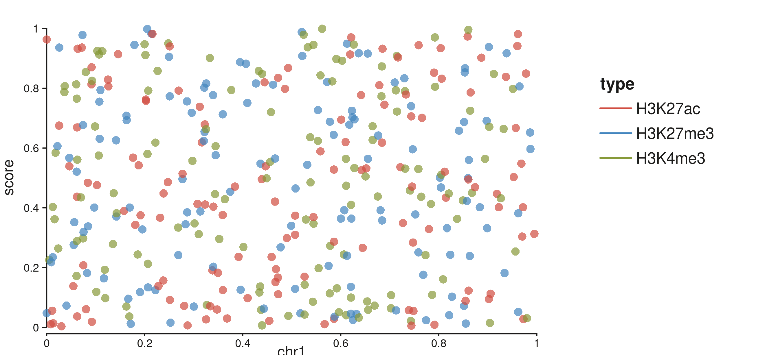

Three-level discrete color legend in the right track margin.

The legend title is taken from the column name. No seq_legend() call is needed.

---

2. Shape auto-legend from map(shape = ...)

map(shape = ...) works the same way for discrete columns. Levels are cycled through circle → square → triangle → diamond, and a matching keyed legend appears in the right margin:

p2 <- seq_plot(aesthetics = right_margin) %+%
  seq_track(data = gr, mapping = map(x = start, y = score), windows = win) %+%
  seq_point(
    aesthetics = aes(size = 0.8, alpha = 0.7),
    mapping    = map(shape = type)
  )
p2$plot()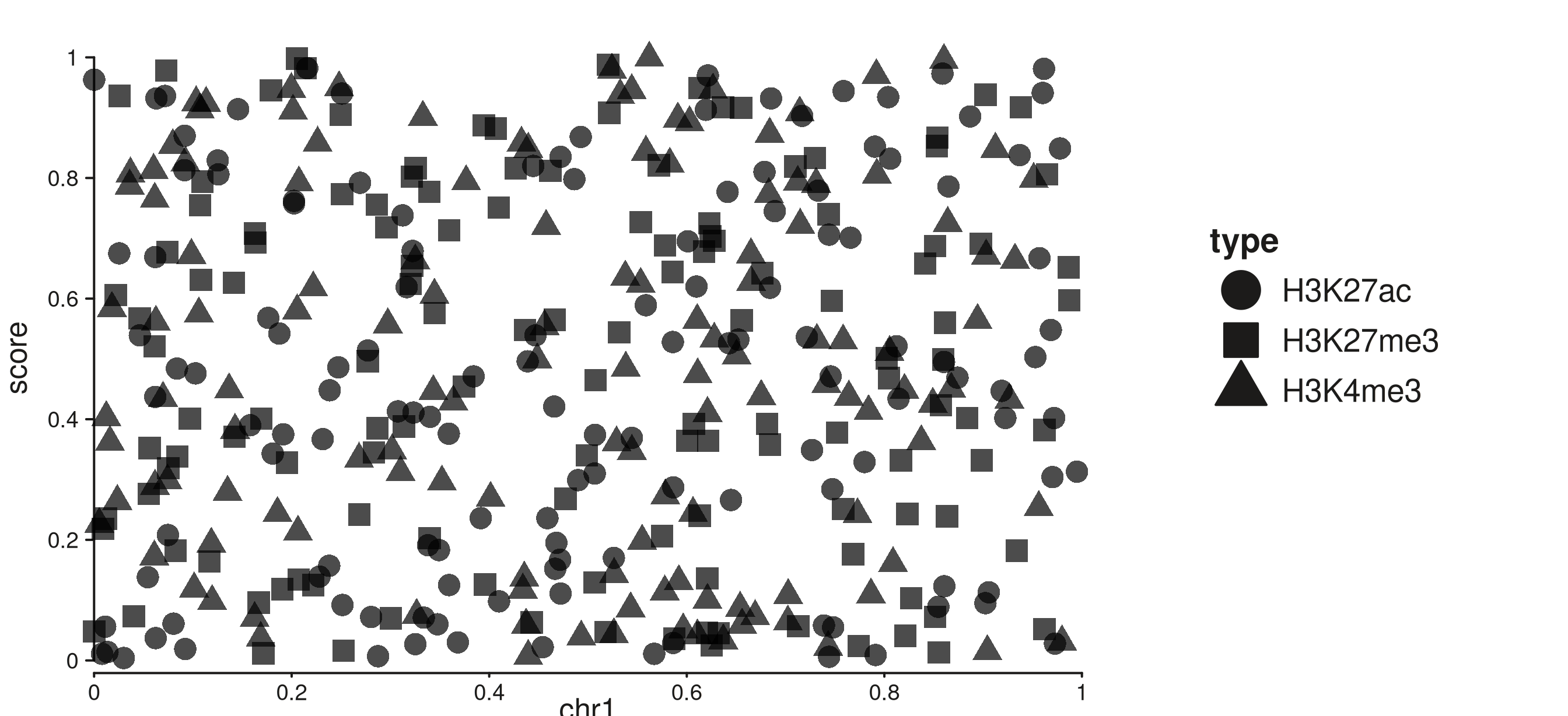

Shape legend auto-generated from map(shape = type) in the right track margin.

---

3. Continuous gradient auto-legend from map(color = ...)

When the mapped column is numeric, SeqPlotR produces a GradientLegendSpec and draws a color bar in the right margin. The viridis palette is used by default. Tick positions are placed automatically with pretty():

p3 <- seq_plot(aesthetics = right_margin) %+%
  seq_track(data = gr, mapping = map(x = start, y = score), windows = win) %+%
  seq_point(
    aesthetics = aes(size = 0.7, alpha = 0.8),
    mapping    = map(color = score)
  )
p3$plot()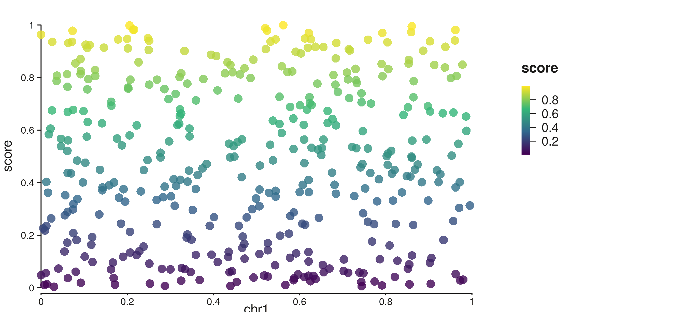

Viridis color bar with auto tick axis in the right track margin.

---

4. Bar chart with discrete fill legend (seq_bar)

seq_bar supports the same auto-legend machinery. Map fill to a discrete column and each group gets a color key in the right margin. The fill values are also automatically scaled to valid colors so bars render correctly:

p4 <- seq_plot(aesthetics = right_margin) %+%
  seq_track(data = gr, mapping = map(x = start, y = score), windows = win) %+%
  seq_bar(
    aesthetics = aes(alpha = 0.85),
    mapping    = map(x = start, y = score, fill = type)
  )
p4$plot()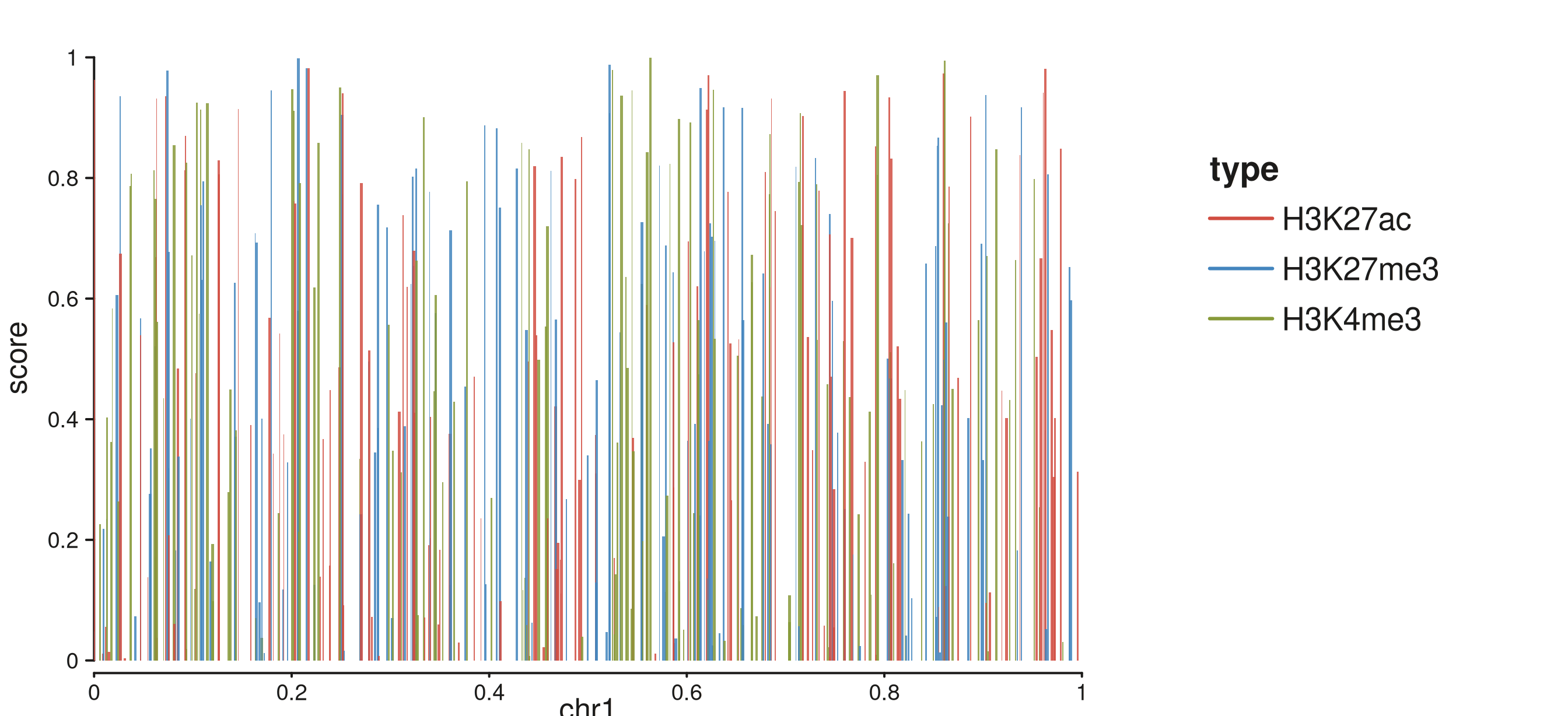

Bar chart with discrete fill auto-legend from map(fill = type).

Map fill to a numeric column and a color-bar legend is produced instead:

p4b <- seq_plot(aesthetics = right_margin) %+%
  seq_track(data = gr, mapping = map(x = start, y = score), windows = win) %+%
  seq_bar(
    aesthetics = aes(alpha = 0.85),
    mapping    = map(x = start, y = score, fill = score)
  )
p4b$plot()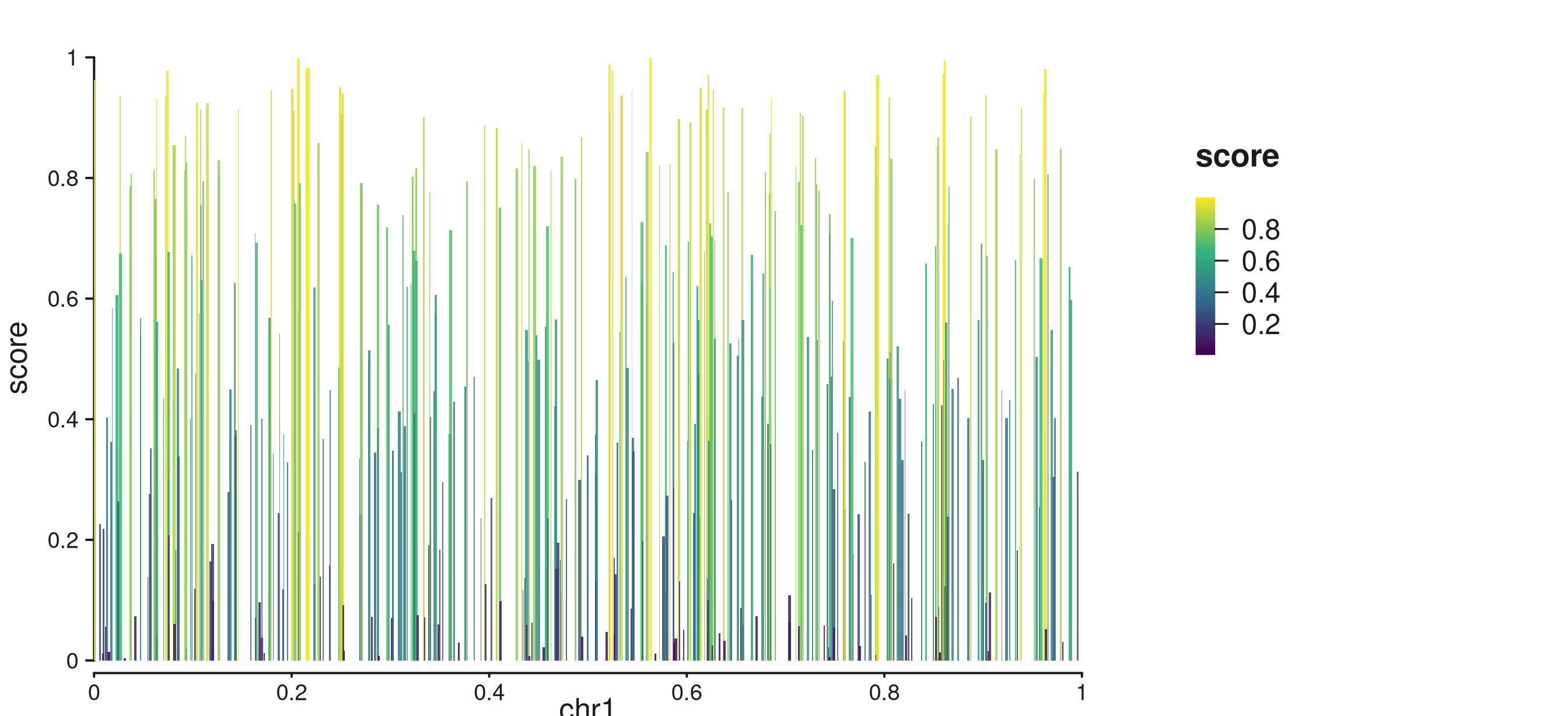

Bar chart with continuous fill gradient auto-legend.

---

5. Line with color legend (seq_line)

seq_line generates an auto-legend from map(color = ...). For discrete columns a keyed legend is placed in the right margin:

p5 <- seq_plot(aesthetics = right_margin) %+%
  seq_track(data = gr, mapping = map(x = start, y = score), windows = win) %+%
  seq_line(
    mapping = map(x = start, y = score, color = type)
  )
p5$plot()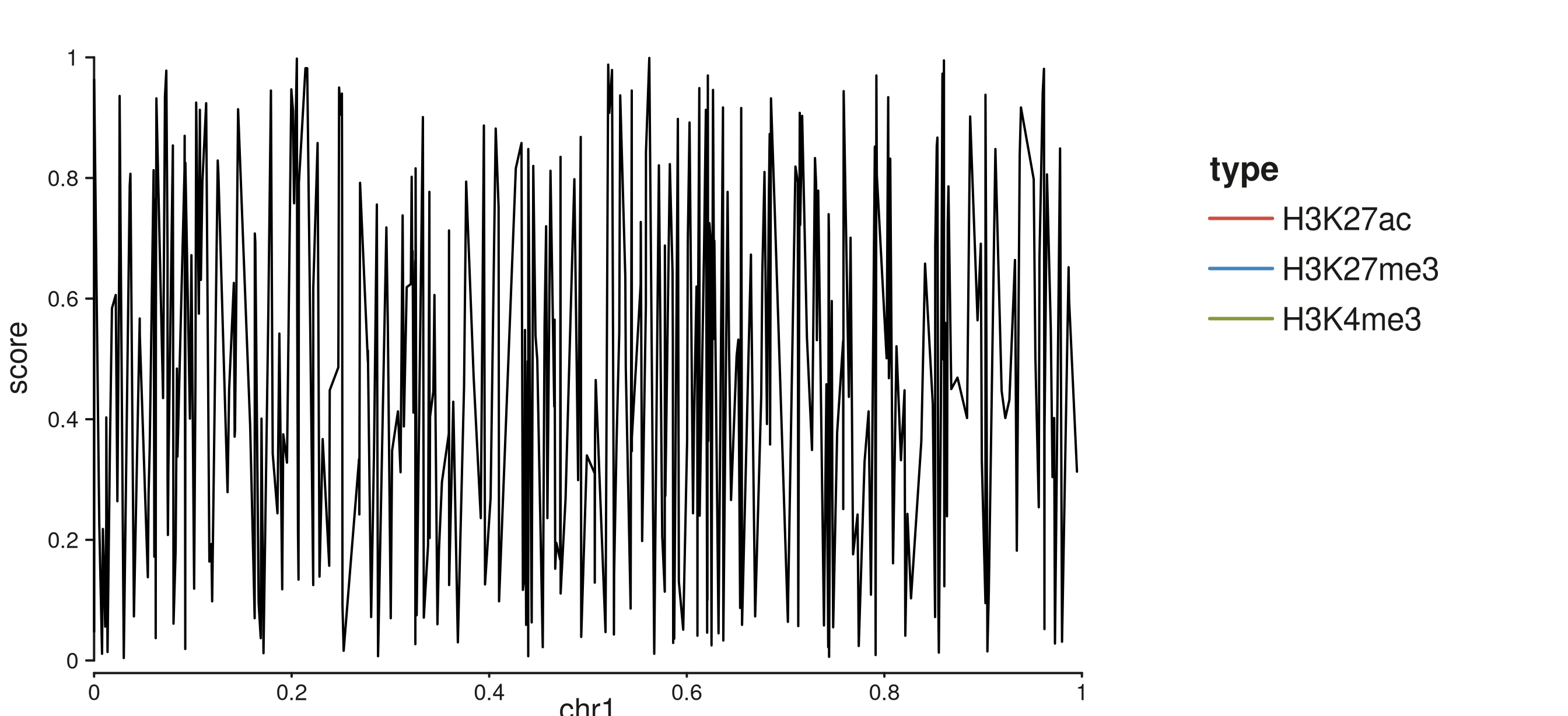

seq_line with discrete color auto-legend.

---

6. Area with fill legend (seq_area)

seq_area generates an auto-legend from map(fill = ...). Map to a numeric column for a gradient legend:

p6 <- seq_plot(aesthetics = right_margin) %+%
  seq_track(data = gr, mapping = map(x = start, y = score), windows = win) %+%
  seq_area(
    mapping = map(x = start, y = score, fill = score)
  )
p6$plot()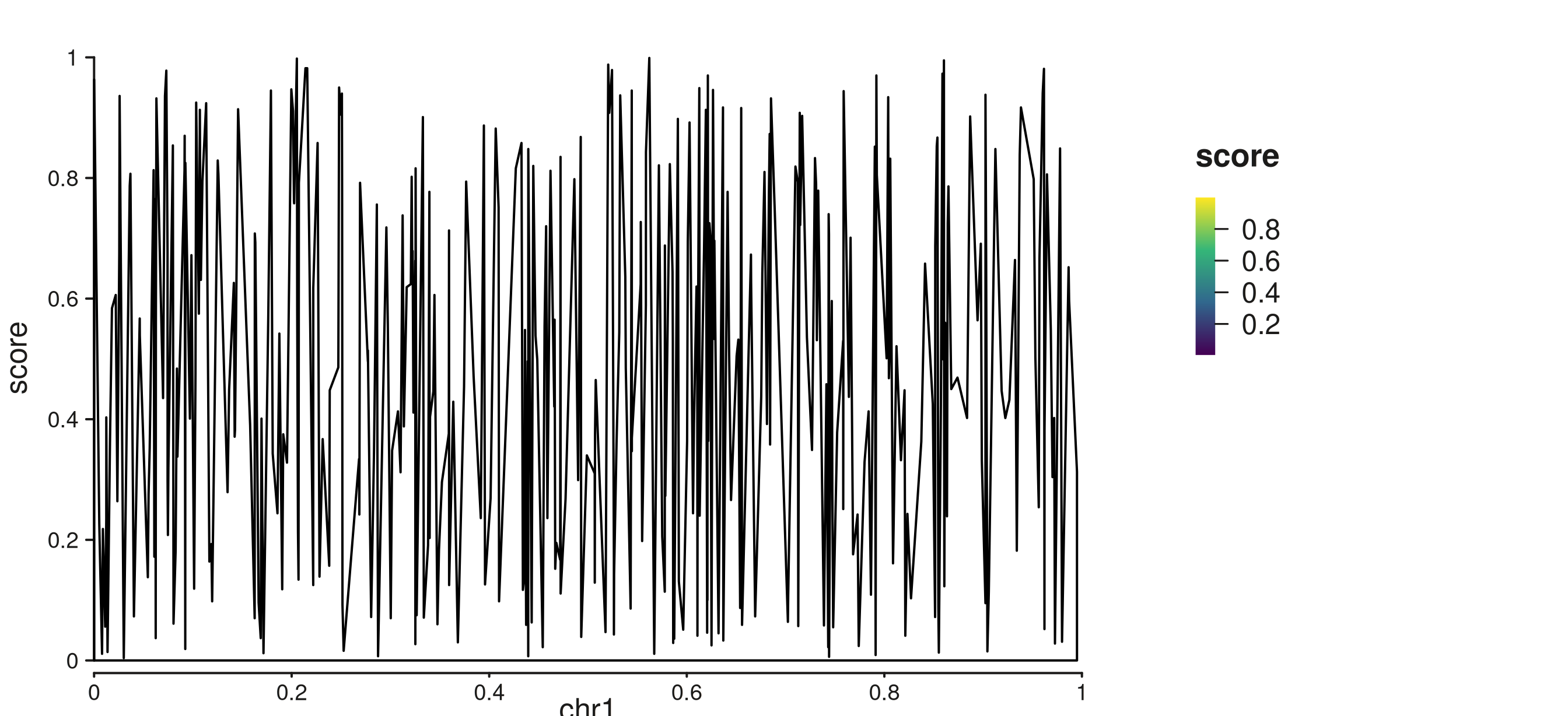

seq_area with continuous fill gradient auto-legend.

---

7. Heatmap with auto fill gradient (seq_tile)

seq_tile also supports auto-scaling. Map fill to a numeric column and a gradient legend with a tick axis is produced automatically:

p7 <- seq_plot(
  aesthetics = aes(margins = list(top = 0.04, bottom = 0.04,
                                   left = 0.04, right = 0.25))
) %+%
  seq_track(windows = win) %+%
  seq_tile(
    data    = gr_tiles,
    mapping = map(x = start, y = y, fill = fill)
  )
p7$plot()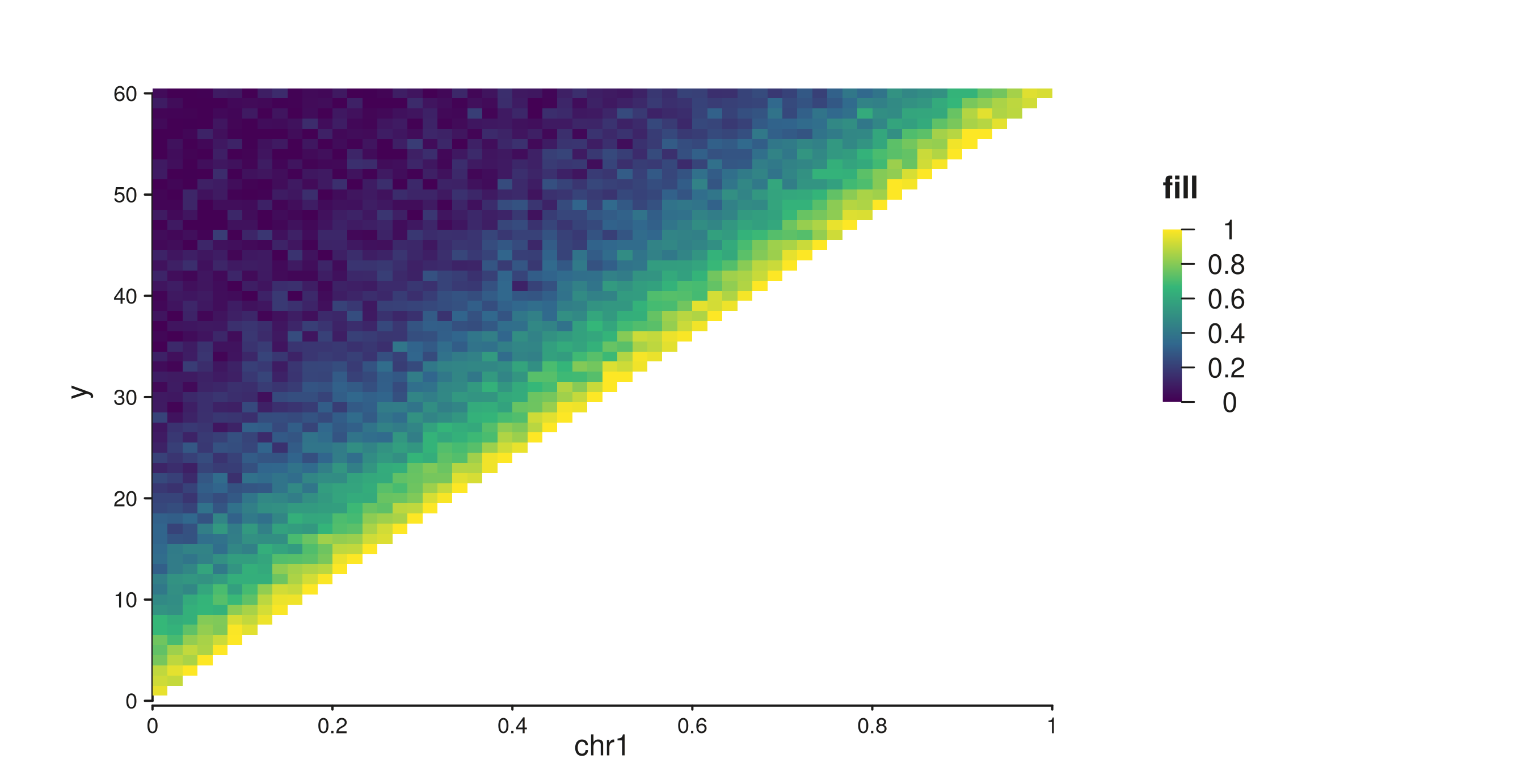

Contact-map tiles with auto gradient legend.

---

8. seq_gradient_legend() — explicit gradient specs

When you need more control — a different palette, specific limits, custom tick positions, or a specific placement — use seq_gradient_legend() directly and attach it to an element via the legend field.

Continuous color bar with a custom palette

breaks = NULL (default) places ticks automatically via pretty().

gleg <- seq_gradient_legend(
  palette  = "plasma",
  limits   = c(0, 1),
  title    = "Score",
  x        = 0.75, y = 0.95,
  position = "inside"
)

p8 <- seq_plot() %+%
  seq_track(data = gr, mapping = map(x = start, y = score), windows = win) %+%
  seq_point(
    mapping    = map(color = score),
    aesthetics = aes(size = 0.7, alpha = 0.8),
    legend     = gleg
  )
p8$plot()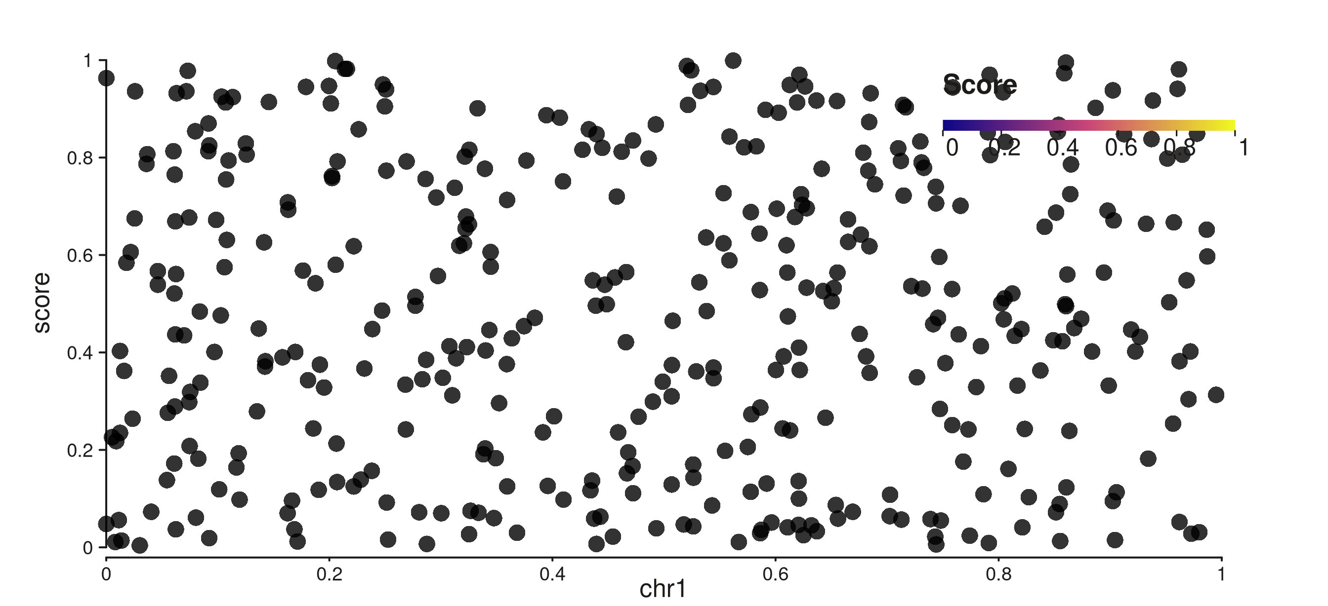

Plasma color bar placed inside the panel at a custom position.

Controlling tick positions

Set breaks to an integer n to place n ticks from pretty(), or supply a numeric vector for exact tick positions. All modes render a continuous color bar with a tick+label axis:

gleg_breaks <- seq_gradient_legend(
  palette     = "viridis",
  limits      = c(0, 1),
  title       = "Score",
  breaks      = 5,
  orientation = "vertical",
  x           = 0.02, y = 0.95,
  position    = "inside"
)

p9 <- seq_plot() %+%
  seq_track(data = gr, mapping = map(x = start, y = score), windows = win) %+%
  seq_point(
    mapping    = map(color = score),
    aesthetics = aes(size = 0.7, alpha = 0.8),
    legend     = gleg_breaks
  )
p9$plot()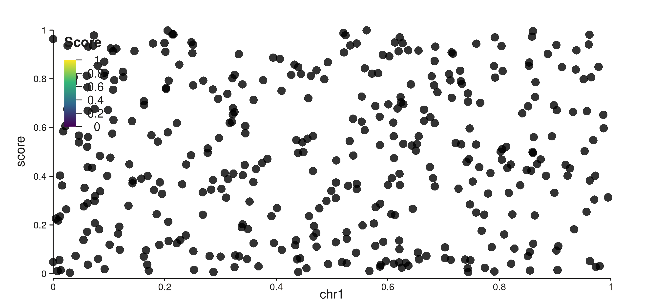

Color bar placed inside with 5 evenly-spaced ticks.

Explicit tick values:

gleg_vals <- seq_gradient_legend(
  palette  = "reds",
  limits   = c(0, 1),
  title    = "Score",
  breaks   = c(0.2, 0.5, 0.8),
  x        = 0.02, y = 0.95,
  position = "inside"
)

p10 <- seq_plot() %+%
  seq_track(data = gr, mapping = map(x = start, y = score), windows = win) %+%
  seq_point(
    mapping    = map(color = score),
    aesthetics = aes(size = 0.7, alpha = 0.8),
    legend     = gleg_vals
  )
p10$plot()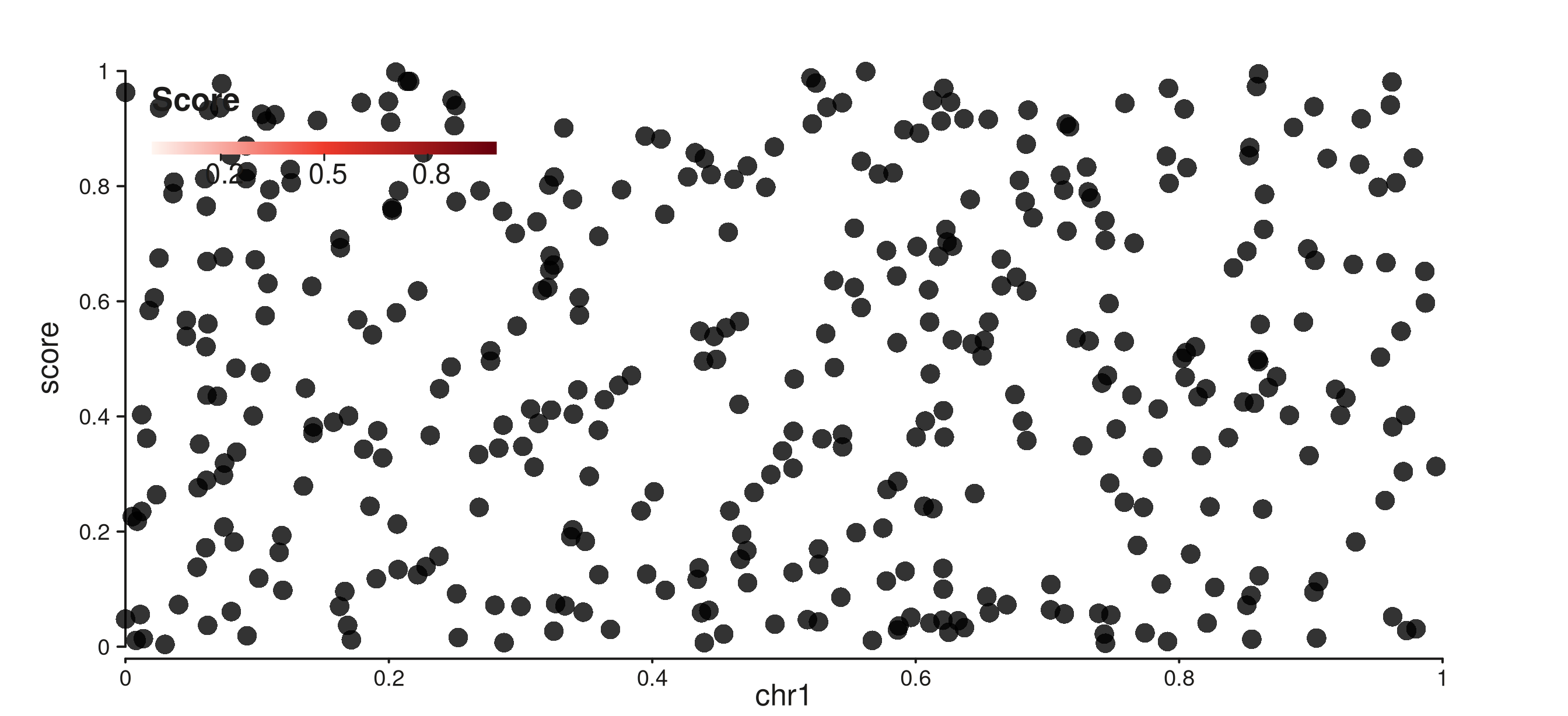

Reds color bar with ticks at 0.2, 0.5, and 0.8.

---

9. Heatmap with a labelled gradient legend

Attach seq_gradient_legend() with breaks to a seq_tile element to get a labelled color bar on a contact-map style heatmap:

hleg <- seq_gradient_legend(
  palette     = "reds",
  limits      = c(0, 1),
  title       = "Contact\nfrequency",
  breaks      = 4,
  x           = 0.72, y = 0.95,
  orientation = "vertical",
  position    = "inside"
)

p11 <- seq_plot(
  aesthetics = aes(margins = list(top = 0.04, bottom = 0.04,
                                   left = 0.04, right = 0.04))
) %+%
  seq_track(windows = win) %+%
  seq_tile(
    data    = gr_tiles,
    mapping = map(x = start, y = y, fill = fill),
    legend  = hleg
  )
p11$plot()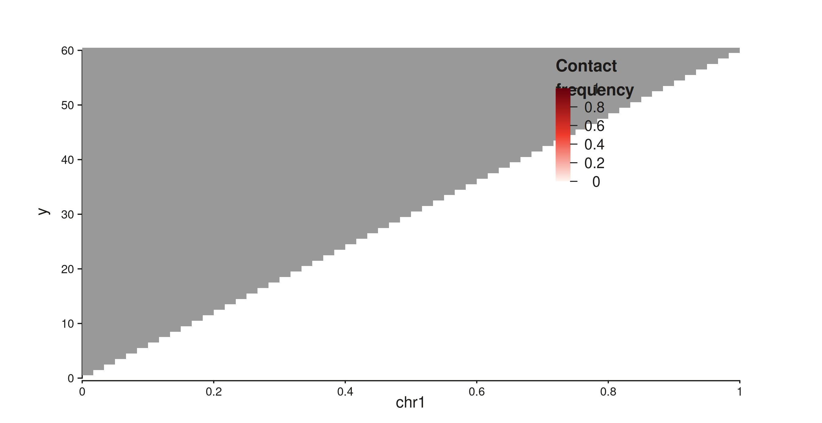

Contact-map heatmap with a four-tick gradient legend placed inside.

---

10. Suppression

Auto-legends respect the same suppression hierarchy as manual legends.

show_legend = FALSE on an element suppresses auto-legend generation:

el_hidden <- seq_point(
  data        = gr,
  mapping     = map(x = start, y = score, color = type),
  show_legend = FALSE
)
# auto_legend is NULL — nothing was generated
is.null(el_hidden$auto_legend)
#> [1] TRUE

seq_plot(legend = FALSE) suppresses all legends including auto-legends:

p_none <- seq_plot(legend = FALSE, aesthetics = right_margin) %+%
  seq_track(data = gr, mapping = map(x = start, y = score), windows = win) %+%
  seq_point(
    mapping    = map(color = type),
    aesthetics = aes(size = 0.6, alpha = 0.7)
  )
p_none$plot()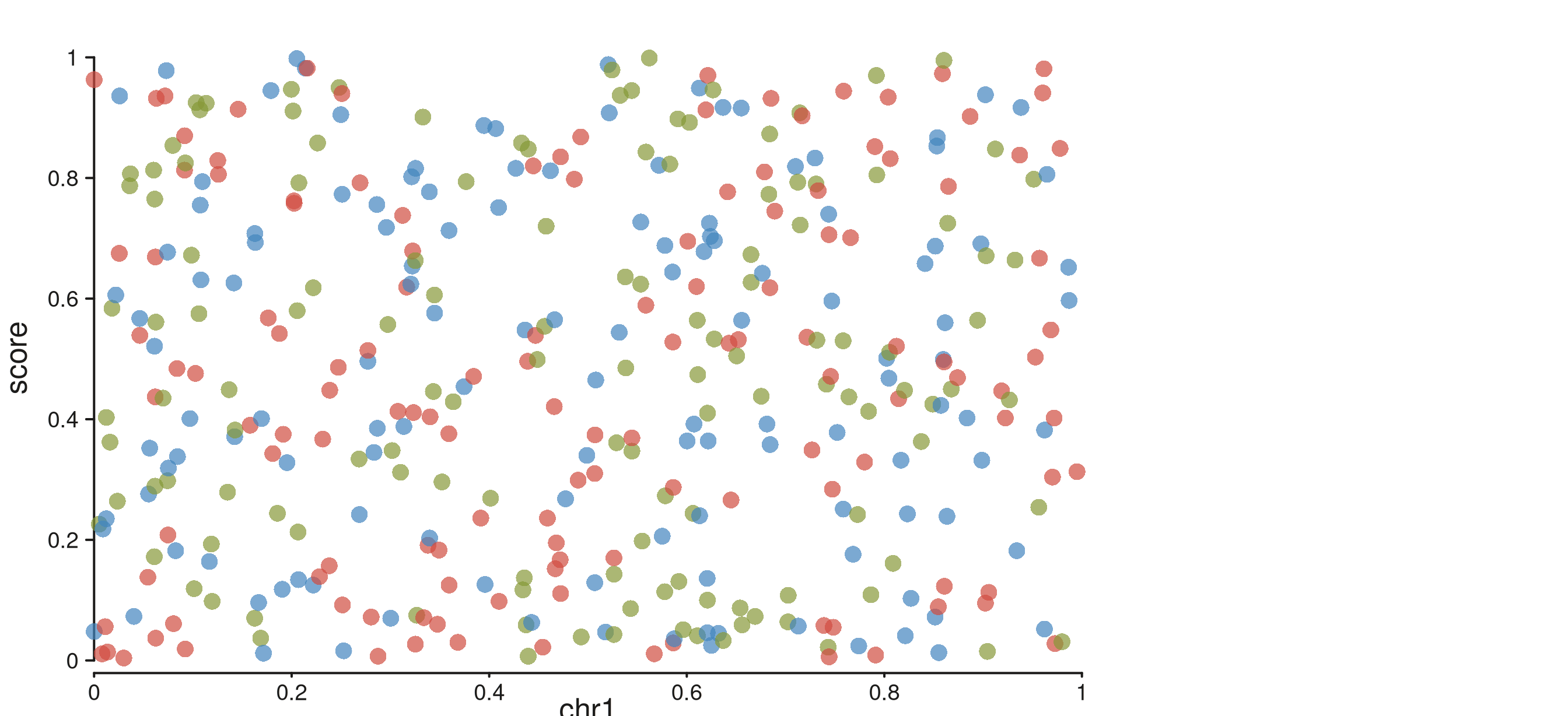

legend = FALSE suppresses the auto-generated discrete legend.

---

Summary

Scenario	How
Discrete auto-legend (color or fill)	map(color = char_col) — no extra call
Shape auto-legend	map(shape = char_col) — no extra call
Continuous gradient auto-legend	map(color = numeric_col) — no extra call
Auto-legend on bar / line / area	seq_bar/line/area(mapping = map(fill = col))
Custom gradient palette / position	legend = seq_gradient_legend(palette=, limits=, ...)
Custom tick positions on colorbar	seq_gradient_legend(breaks = n) or breaks = c(v1, v2, ...)
Suppress auto-legend for one element	seq_point(..., show_legend = FALSE)
Suppress all legends	seq_plot(legend = FALSE)

Auto-legends default to position = "track_margin", side = "right". Set right in the plot margins (aes(margins = list(right = 0.25, ...))) to reserve space for them.

Palette name	Colors
"viridis"	purple → teal → yellow (default)
"plasma"	dark blue → magenta → yellow
"magma"	black → red → cream
"blues"	white → mid blue → navy
"reds"	white → red → dark red