New features: expansion, OOB, titles, margins, inheritance

library(SeqPlotR)
library(GenomicRanges)

This vignette covers the cross-cutting feature batch that touches scales, axes, margins, and the Hi-C fetcher:

Axis expansion now actually applies to element coordinates.
New oob = "exclude" / "perimeter" argument on every scale.
aes(axis.x.line = NA) removes a piece of axis chrome, ggplot-style.
Axis titles auto-derive from the first element’s mapping.
Genomic axes default each window’s title to its seqname.
Manual title overrides via axis.<side>.title.label / axis.<side>.title = aes(label = …, col = …).
New pretty = list(...) argument forwards to base pretty().
seq_plot(windows = …) is inherited by tracks; genomic scales inherit windows from their enclosing track.
New seq_plot(plot_margin = 0.02) outermost canvas margin.
New seq_plot(highlight_margins = TRUE) development overlay.
open_hic()$fetch() now accepts a multi-range region; the max_fetch_bp default raised to 280 Mb.

We use a synthetic two-track example throughout. The data:

win <- GRanges("chr1", IRanges(start = 1, end = 1e6))
n   <- 200
gr  <- GRanges("chr1", IRanges(start = sample(1:1e6, n), width = 1))
mcols(gr)$xv    <- runif(n, 0, 10)
mcols(gr)$score <- runif(n, 0, 6)
mcols(gr)$grp   <- sample(letters[1:3], n, TRUE)

1. Axis expansion (now wired through)

Previously, passing expand = c(0.1, 0) on a continuous scale had no visible effect — the breaks were computed but the npc transform that positions data on the panel used the raw data range. As of this batch, expand is honoured end-to-end: the panel carries an xplot_range / yplot_range that includes the expansion, and elements map into it.

trk_noexp <- seq_track(
  data    = gr, windows = win,
  mapping = map(x = xv, y = score),
  scale_x = seq_scale_continuous(expand = c(0,   0)),
  aesthetics = aes("axis.x.title.label" = "x (no expand)")
) %+% seq_point()

trk_exp <- seq_track(
  data    = gr, windows = win,
  mapping = map(x = xv, y = score),
  scale_x = seq_scale_continuous(expand = c(0.2, 0)),
  aesthetics = aes("axis.x.title.label" = "x (20% expansion)")
) %+% seq_point()

(seq_plot() %+% trk_noexp %+% trk_exp)$plot()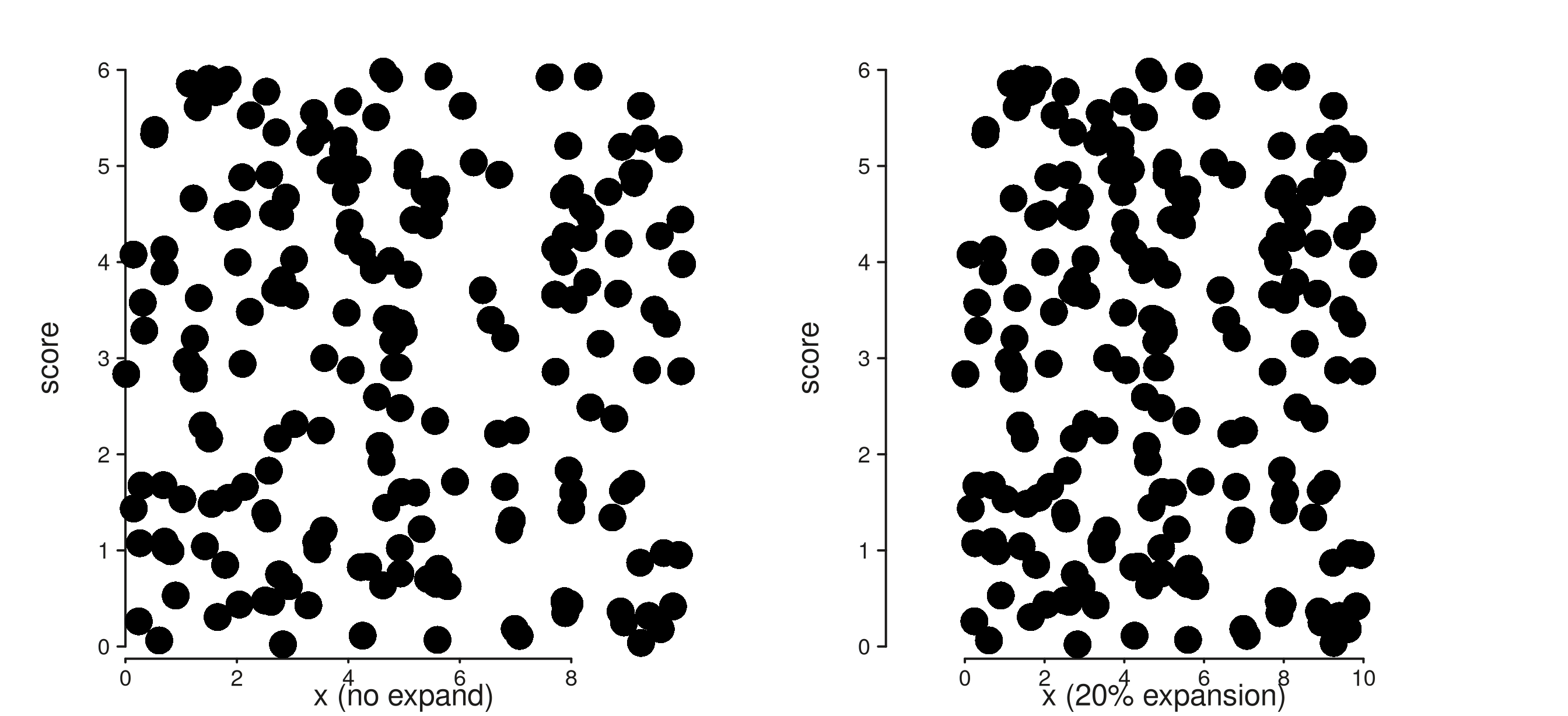

2. `oob` — out-of-bounds handling

The new oob argument controls what happens when data falls outside the (expanded) axis range. "exclude" (default) drops the rows and reports a count via message(); "perimeter" clamps them to the limit and reports.

# A subset whose x runs from -3 to 13 — three points sit outside [0, 10].
gr_off <- gr
mcols(gr_off)$xv <- jitter(c(-3, mcols(gr)$xv[2:(n-1)], 13), amount = 1)

trk_excl <- seq_track(
  data    = gr_off, windows = win,
  mapping = map(x = xv, y = score),
  scale_x = seq_scale_continuous(limits = c(0, 10), oob = "exclude"),
  aesthetics = aes("axis.x.title.label" = "oob = exclude")
) %+% seq_point()

trk_per <- seq_track(
  data    = gr_off, windows = win,
  mapping = map(x = xv, y = score),
  scale_x = seq_scale_continuous(limits = c(0, 10), oob = "perimeter"),
  aesthetics = aes("axis.x.title.label" = "oob = perimeter")
) %+% seq_point()

(seq_plot() %+% trk_excl %+% trk_per)$plot()
#> 4 out-of-bounds data points excluded! (seq_point)
#> 4 out-of-bounds data points plotted! (seq_point)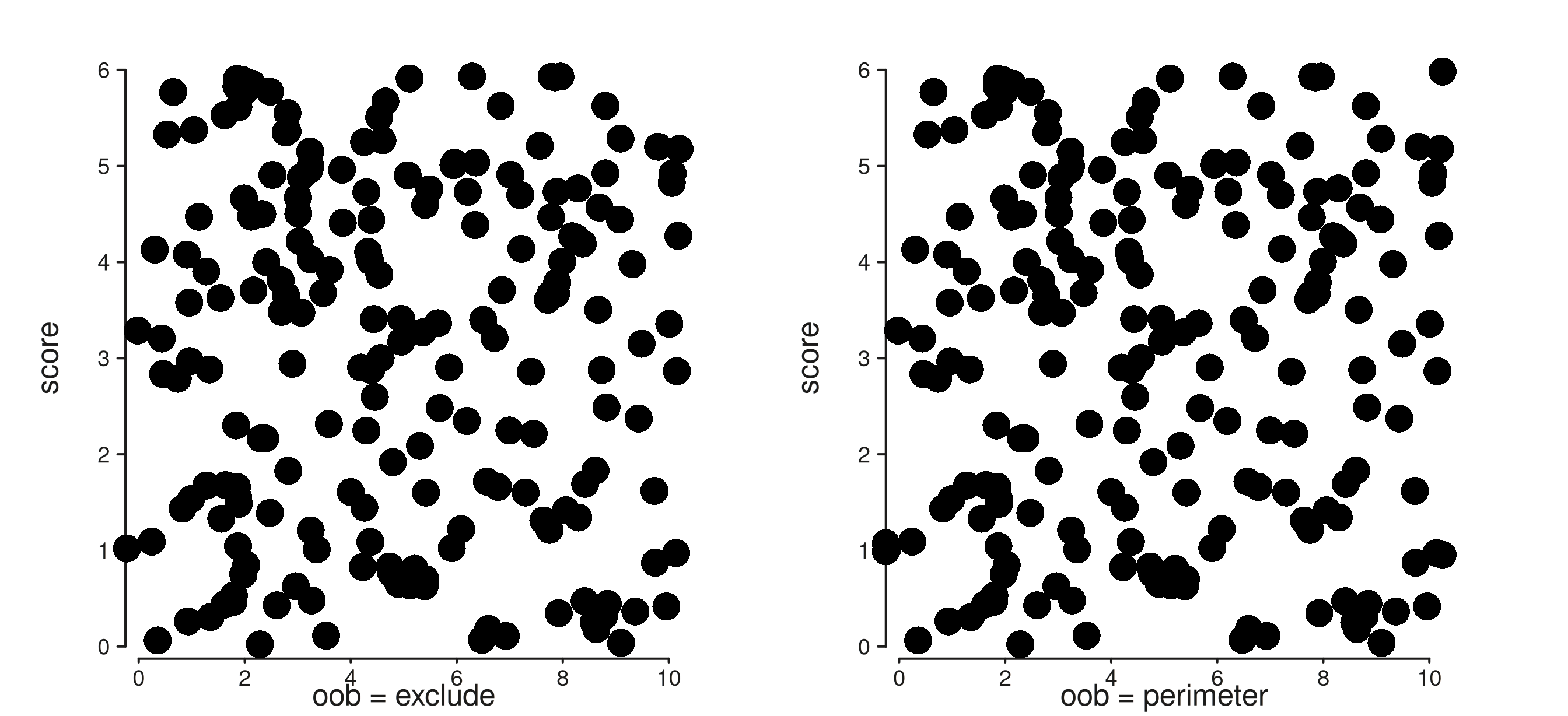

3. `NA` removes axis chrome

Setting any of the structural axis sub-keys (line, title, ticks, labels, text, gridline) to NA blanks that piece — the same contract as ggplot’s element_blank(). Sides x / y (default both), x1 / x2 / y1 / y2 (specific axis), and the top-level axis.* (every axis) all work.

trk_full <- seq_track(
  data = gr, windows = win,
  mapping = map(x = xv, y = score)
) %+% seq_point()

trk_no_line_no_ticks <- seq_track(
  data = gr, windows = win,
  mapping = map(x = xv, y = score),
  aesthetics = aes(
    "axis.x.line"  = NA,
    "axis.x.ticks" = NA,
    "axis.x.text"  = NA
  )
) %+% seq_point()

(seq_plot() %+% trk_full %+% trk_no_line_no_ticks)$plot()

4 & 5 & 6. Smarter axis titles

The default axis title now derives from the first element’s mapping (falling back to the track’s mapping, then to the seqname when the scale is genomic). You can override with a plain string label or a styled aes(label = ..., col = ..., size = ...).

# Element mapping wins over track mapping for the title.
trk_a <- seq_track(data = gr, windows = win) %+%
         seq_point(mapping = map(x = xv, y = score))

# Manual override via the convenience .label sub-key.
trk_b <- seq_track(data = gr, windows = win,
                   mapping    = map(x = xv, y = score),
                   aesthetics = aes("axis.x.title.label" = "Custom title")) %+%
         seq_point()

# Or a full styled aes — sets label and any nested style keys at once.
trk_c <- seq_track(
  data       = gr, windows = win,
  mapping    = map(x = xv, y = score),
  aesthetics = aes(axis.x.title = aes(label = "Styled title",
                                       col   = "#A0282C",
                                       size  = 1.0))
) %+% seq_point()

(seq_plot() %+% trk_a %+% trk_b %+% trk_c)$plot()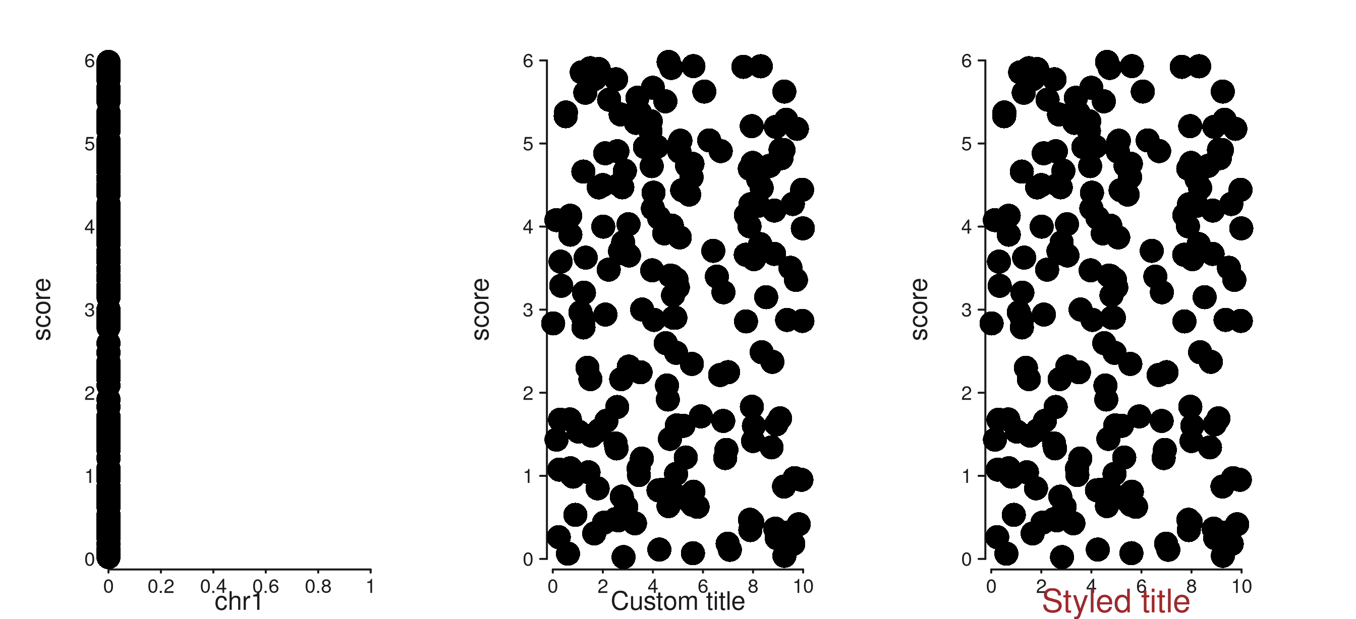

Genomic axes (seq_scale_genomic(), or the auto-built genomic scale when the user supplies no scale_x) get a per-window seqname as the default title:

multi_win <- GRanges(
  c("chr1", "chr2", "chr3"),
  IRanges(start = c(1, 1, 1), end = c(1e6, 1e6, 1e6))
)
multi_data <- GRanges(
  rep(c("chr1", "chr2", "chr3"), each = 50),
  IRanges(start = c(sample(1:1e6, 50),
                    sample(1:1e6, 50),
                    sample(1:1e6, 50)), width = 1)
)
mcols(multi_data)$score <- runif(150, 0, 5)

trk_multi <- seq_track(
  data    = multi_data, windows = multi_win,
  mapping = map(y = score)
) %+% seq_point()

(seq_plot() %+% trk_multi)$plot()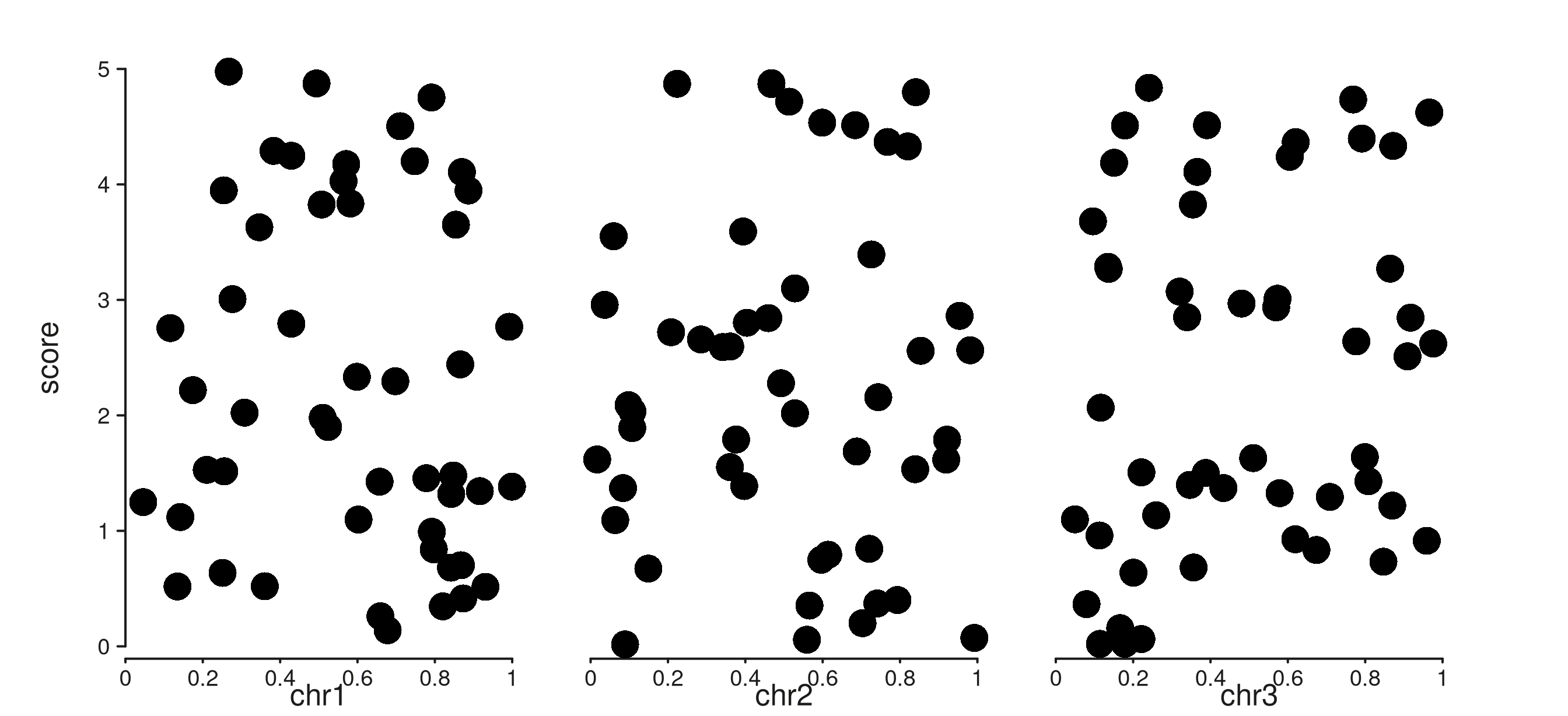

7. `pretty = list(...)`

All position scales now accept a pretty argument: a named list of additional arguments forwarded to base pretty().

trk_default <- seq_track(
  data = gr, windows = win,
  mapping    = map(x = xv, y = score),
  scale_x    = seq_scale_continuous(limits = c(0, 10)),
  aesthetics = aes("axis.x.title.label" = "default n_breaks = 5")
) %+% seq_point()

trk_pretty <- seq_track(
  data = gr, windows = win,
  mapping    = map(x = xv, y = score),
  scale_x    = seq_scale_continuous(
                  limits = c(0, 10),
                  pretty = list(n = 10, min.n = 5)),
  aesthetics = aes("axis.x.title.label" = "pretty = list(n = 10, min.n = 5)")
) %+% seq_point()

(seq_plot() %+% trk_default %+% trk_pretty)$plot()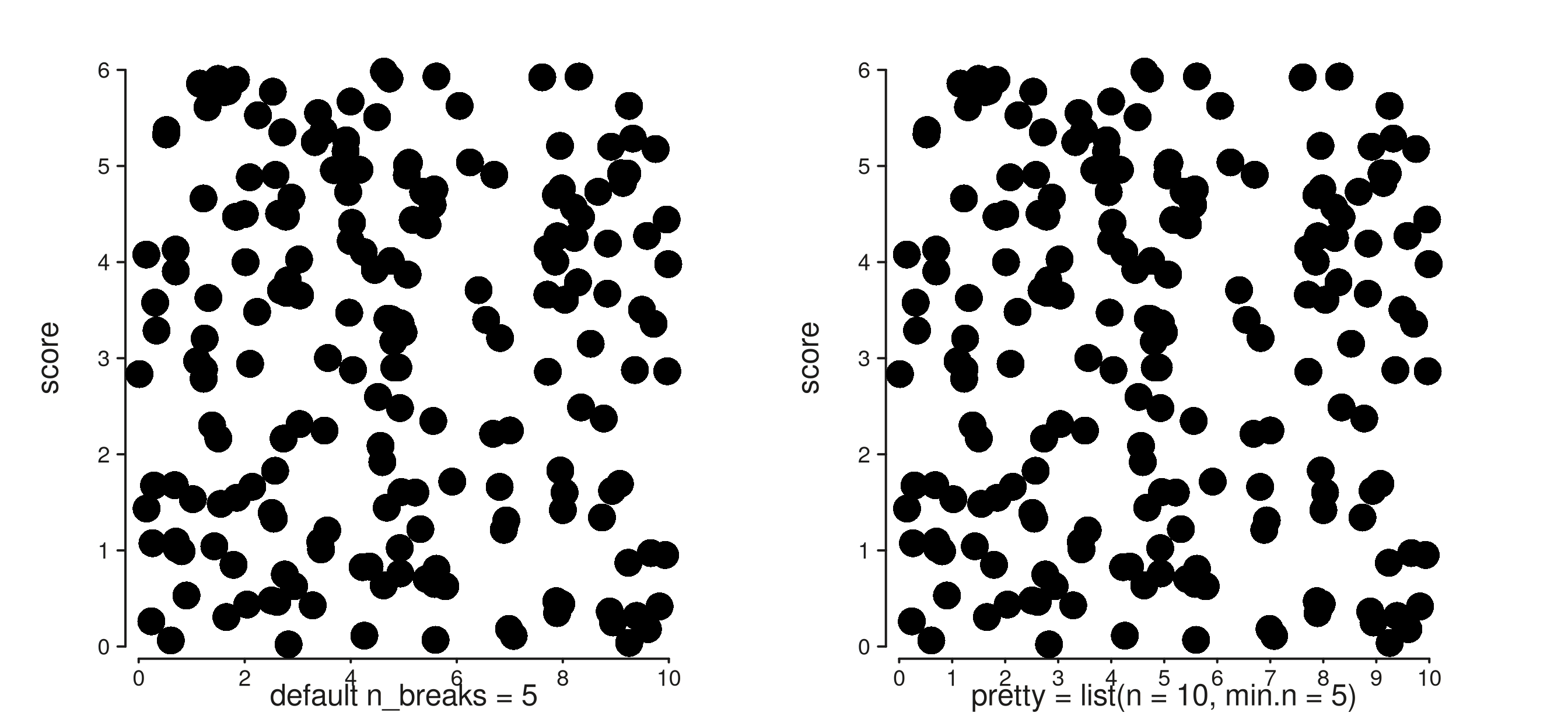

8. Windows inheritance

seq_plot() accepts a windows argument that any track without its own windows inherits. Genomic scales constructed without explicit windows inherit from the enclosing track. This trims boilerplate when many tracks share the same windows.

# Old style — every track repeats the windows.
old <- seq_plot() %+%
  (seq_track(data = gr, windows = win,
             mapping = map(x = xv, y = score)) %+% seq_point()) %+%
  (seq_track(data = gr, windows = win,
             mapping = map(x = xv, y = score)) %+% seq_point())

# New style — windows live on the plot.
new <- seq_plot(windows = win) %+%
  (seq_track(data = gr,
             mapping = map(x = xv, y = score)) %+% seq_point()) %+%
  (seq_track(data = gr,
             mapping = map(x = xv, y = score)) %+% seq_point())

new$plot()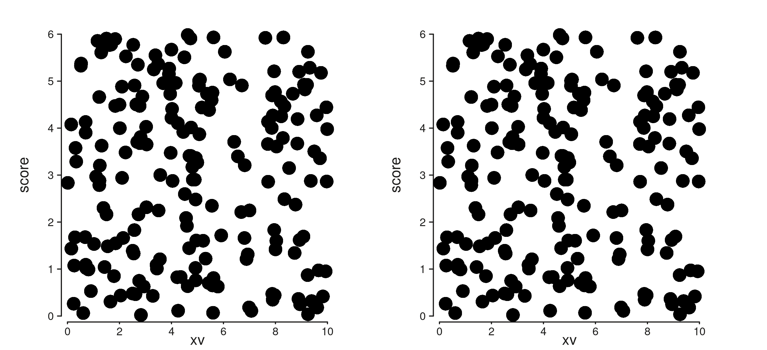

Genomic scales also pick up the enclosing track’s windows when constructed bare:

trk_bare_scale <- seq_track(
  data    = gr, windows = win,
  scale_x = seq_scale_genomic()           # no windows arg
) %+% seq_point()

(seq_plot() %+% trk_bare_scale)$plot()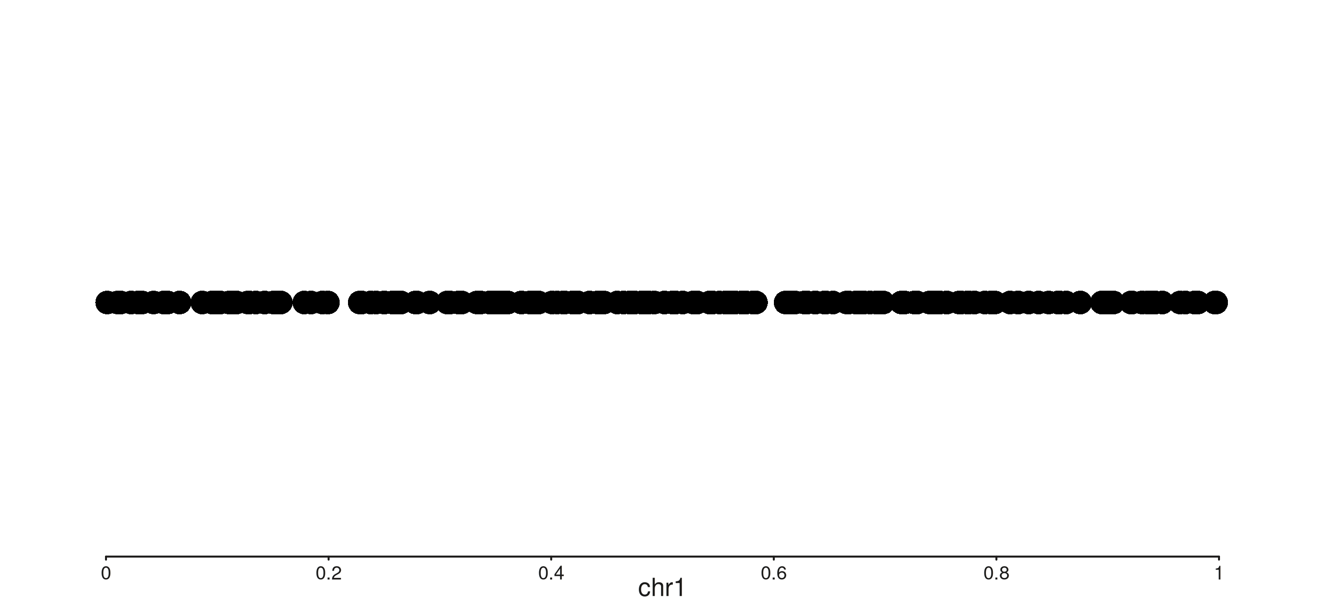

9. `plot_margin`

seq_plot(plot_margin = 0.02) sets the outermost canvas margin (in NPC units). The default is 0.02. Per-side overrides via aesthetics = aes(margins = list(top = ..., ...)) still win.

tight  <- seq_plot(plot_margin = 0,    windows = win) %+%
          (seq_track(data = gr,
                     mapping = map(x = xv, y = score)) %+% seq_point())
roomy  <- seq_plot(plot_margin = 0.08, windows = win) %+%
          (seq_track(data = gr,
                     mapping = map(x = xv, y = score)) %+% seq_point())

tight$plot()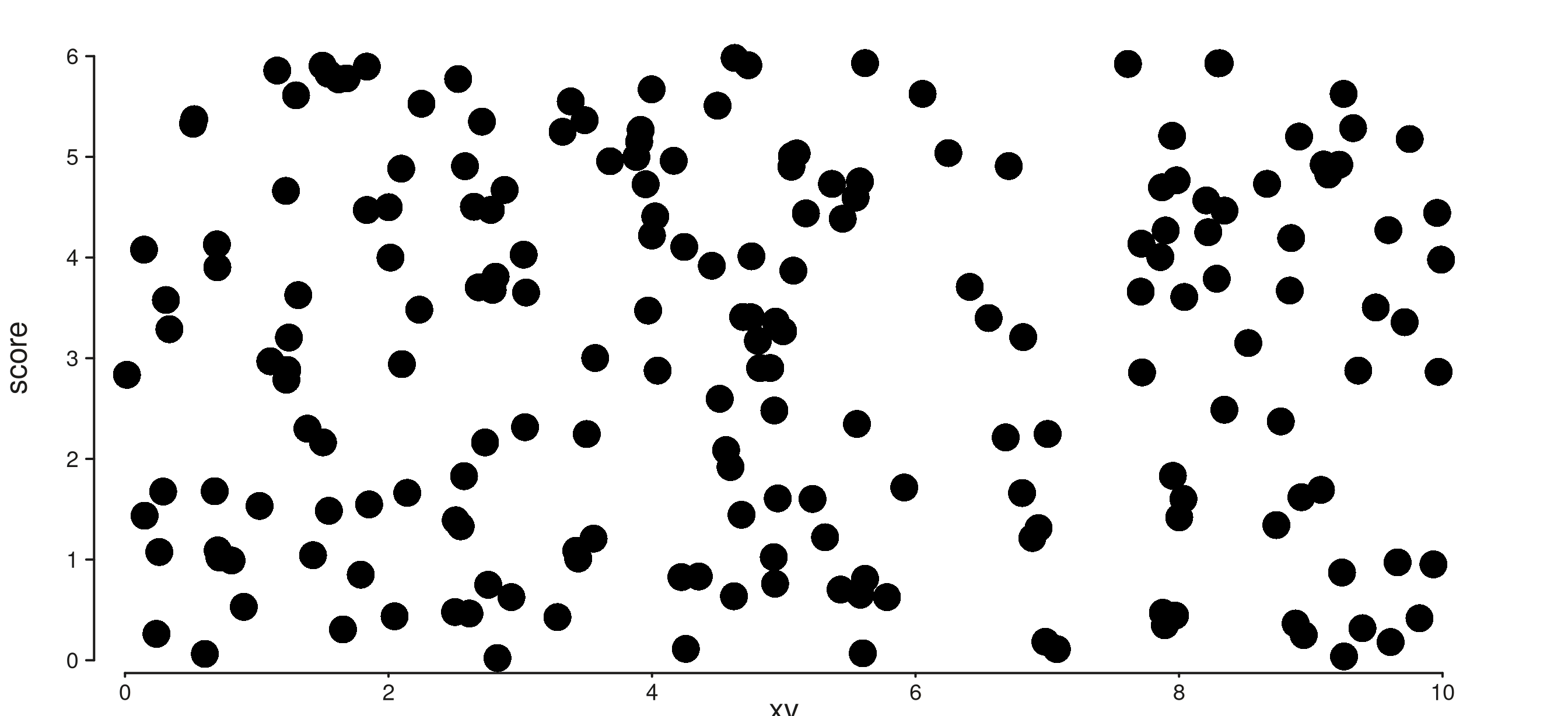

roomy$plot()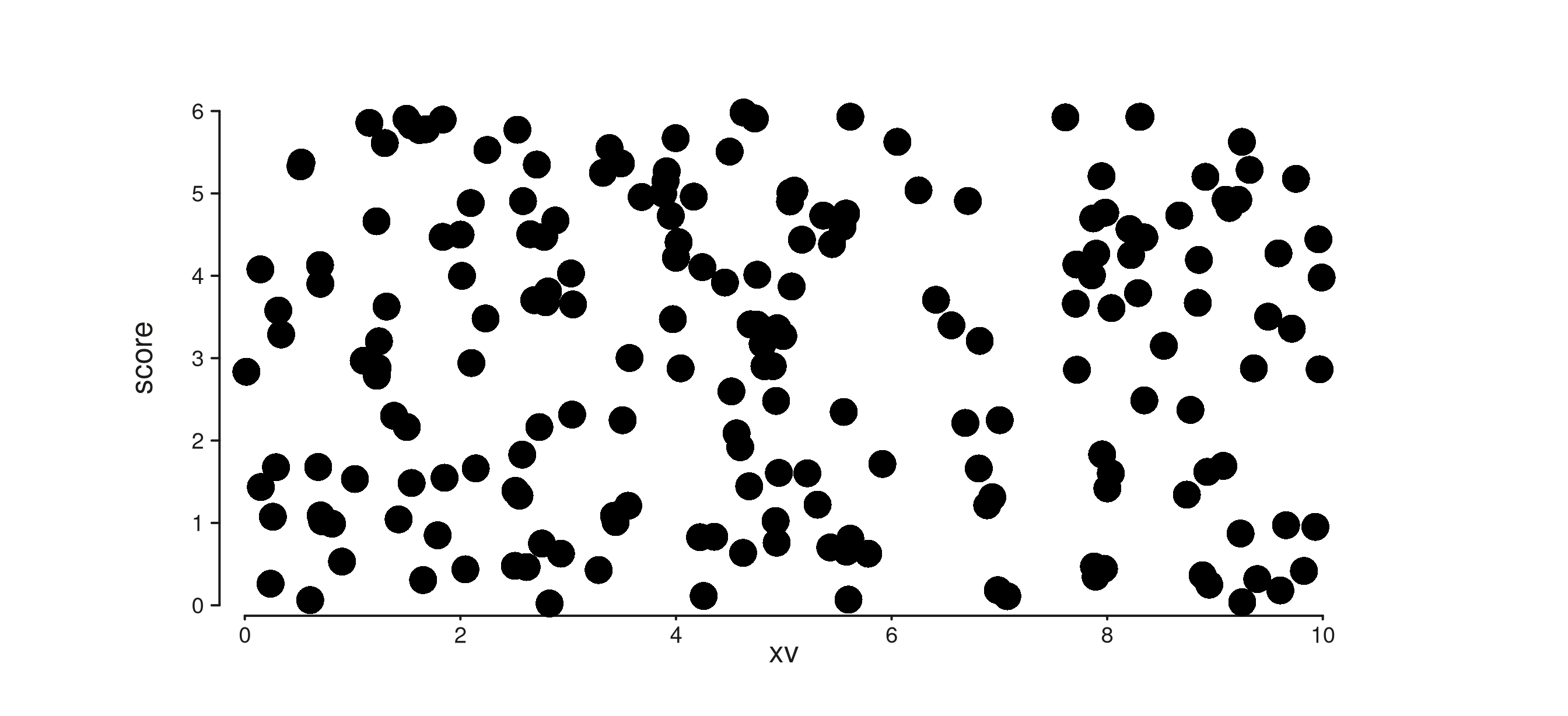

10. `highlight_margins` — development overlay

A development aid: setting highlight_margins = TRUE overlays translucent rectangles on every margin band. Useful when tuning the layout or chasing a stray gap.

highlighted <- seq_plot(windows = win, highlight_margins = TRUE, plot_margin = 0.05) %+%
  (seq_track(data = gr,
             mapping = map(x = xv, y = score),
             track_outer_margin  = 0.04,
             track_inner_margin  = 0.03,
             window_outer_margin = 0.02,
             window_inner_margin = 0.02) %+%
   seq_point())
highlighted$plot()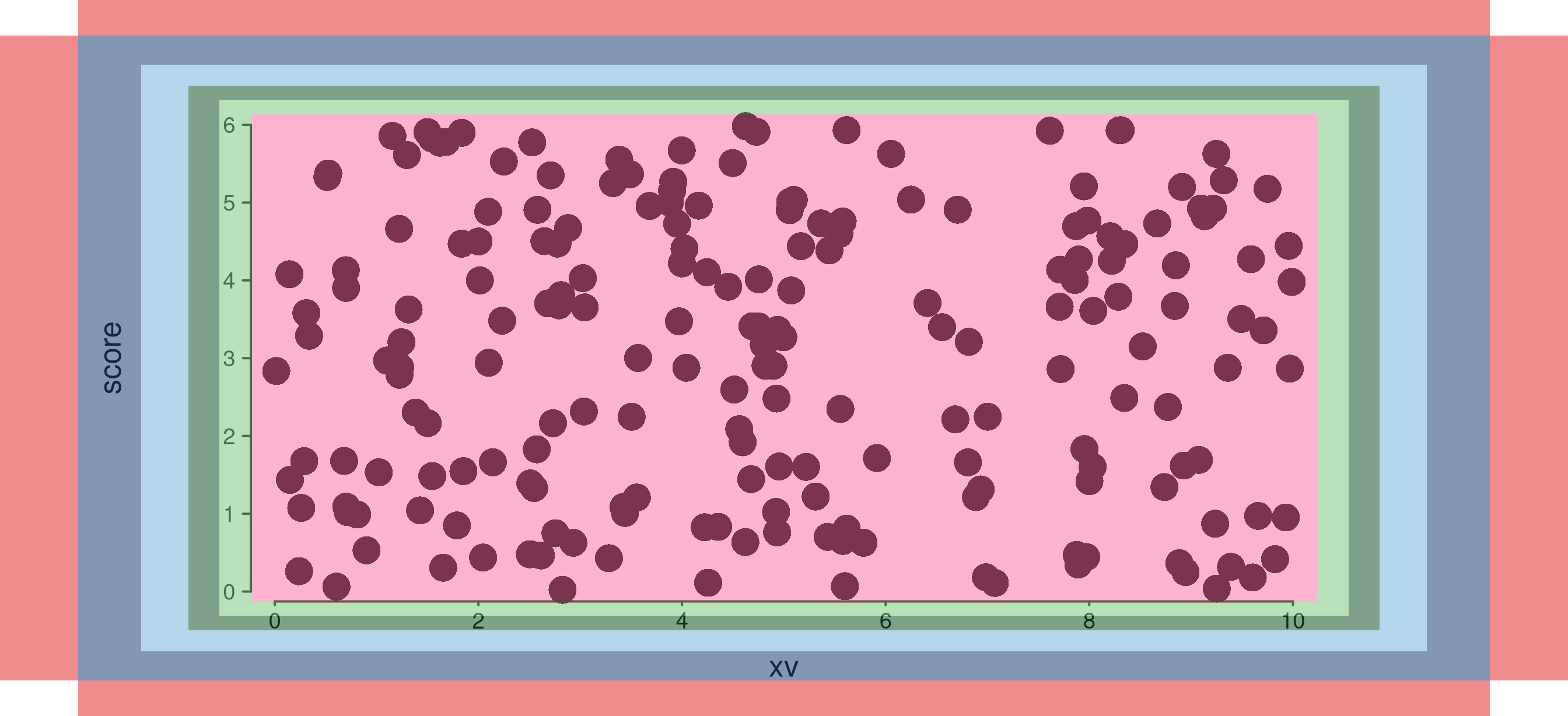

Colours:

Region	Colour
`plot_margin`	red
`track_outer_margin`	dark blue
`track_inner_margin`	light blue
`window_outer_margin`	dark green
`window_inner_margin`	light green
plotting area (`inner`)	pink

All drawn at alpha = 0.5.

11. Hi-C fetcher: multi-range and 280 Mb default

open_hic()$fetch() now takes a single region GRanges that may contain multiple ranges; each range produces its own intra-region contact submatrix, and the results are concatenated into a single BEDPE data frame. The previous region1 / region2 interface is replaced.

The max_fetch_bp default has been raised from 5 Mb to 280 Mb so whole-chromosome fetches work out of the box; the check now applies per range rather than to the sum.

hic <- open_hic("path/to/file.hic", resolution = 25000L)

# Single range — same as before, but uses the new arg name.
hic$fetch(GRanges("chr14", IRanges(98e6, 99e6)))

# Multi-range fetch in one call.
multi_regions <- GRanges(
  c("chr14", "chr15"),
  IRanges(start = c(98e6, 50e6), end = c(99e6, 51e6))
)
hic$fetch(multi_regions)

Each row in the returned data frame carries the seqname of the range that produced it (seqnames1/seqnames2), so downstream code can still distinguish per-region contacts.

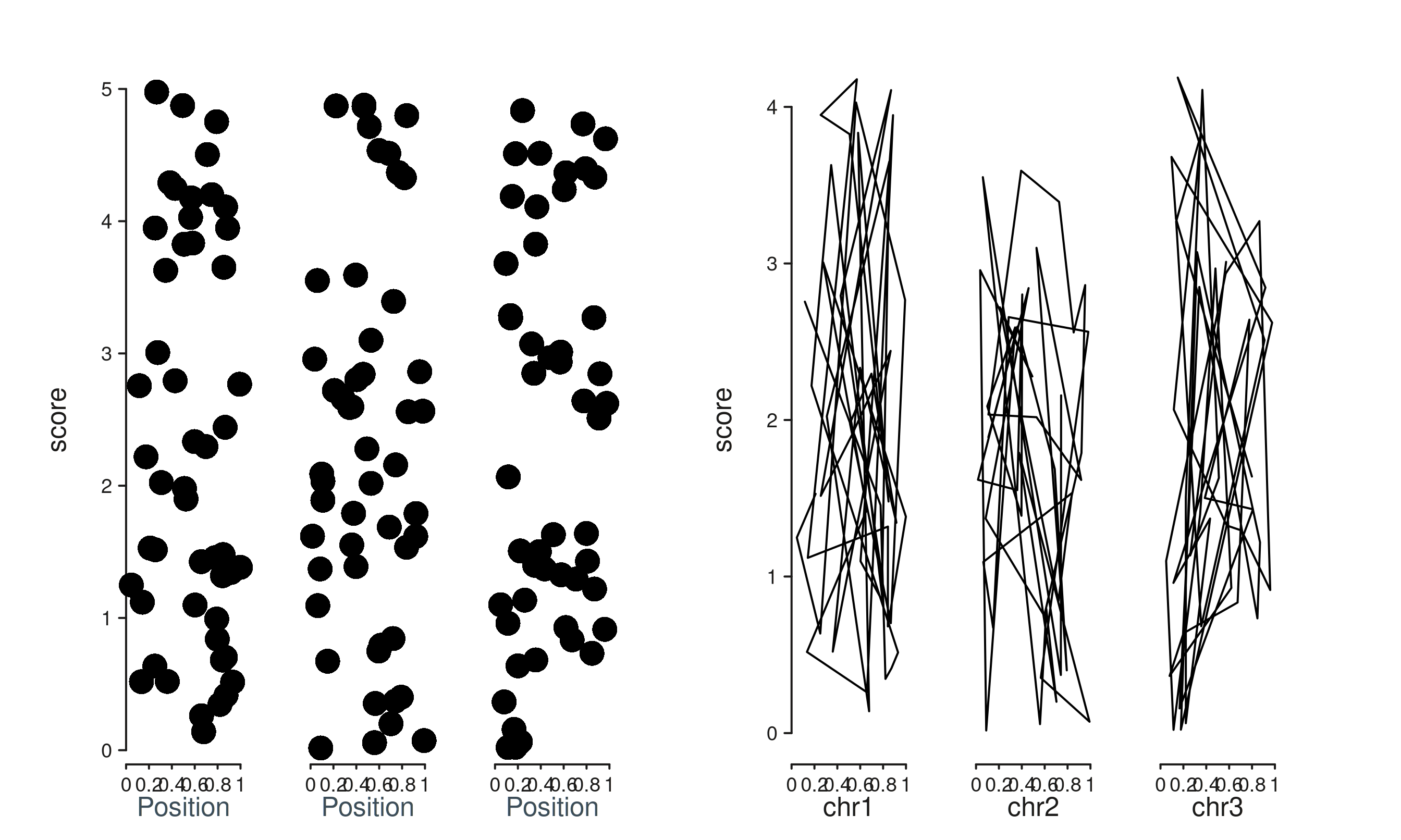
Putting it together

A small showcase that uses several of the new features in one plot:

showcase <- seq_plot(windows = multi_win, plot_margin = 0.03) %+%
  (seq_track(
     data    = multi_data,
     mapping = map(y = score),
     aesthetics = aes(axis.x.title = aes(label = "Position",
                                          col   = "#3D4D58"))
   ) %+% seq_point()) %+%
  (seq_track(
     data    = multi_data,
     mapping = map(x = start, y = score),
     scale_y = seq_scale_continuous(limits = c(0, 4),
                                     expand = c(0.05, 0),
                                     oob    = "exclude",
                                     pretty = list(n = 4))
   ) %+% seq_path())
showcase$plot()
#> 7 out-of-bounds data points excluded! (seq_path)
#> 9 out-of-bounds data points excluded! (seq_path)
#> 9 out-of-bounds data points excluded! (seq_path)

1. Axis expansion (now wired through)

2. oob — out-of-bounds handling

3. NA removes axis chrome