Batch 9: In-panel axes, seq_reads, seq_scalebar, and file connections • SeqPlotR

library(SeqPlotR)
library(GenomicRanges)

Batch 9 introduces six independent feature groups: in-panel axis title / range labels, composable seq_gene label placement, ideogram scope and style options, seq_reads() for IGV-style alignment views, seq_scalebar() for axis-free length references, and a small family of on-demand file connection helpers (open_bigwig(), open_bam(), open_hic()).

In-panel axis titles and range labels

The default behaviour of axes has not changed — titles render in the margin band and per-tick labels stack along the axis. Two new theme keys let you override this on a per-axis basis: axis.<dim>.title.position and axis.<dim>.labels.style / .position.

win <- GRanges("chr1", IRanges(1, 1000))
gr  <- GRanges("chr1", IRanges(c(100, 400, 700), width = 80),
               score = c(1, 3, 2))

p <- seq_plot() %+%
  (seq_track(
     data    = gr, windows = win,
     aesthetics = aes(
       "axis.y.title.text"      = "Score",
       "axis.y.title.position"  = c(0.02, 0.95),
       "axis.y.labels.style"    = "range",
       "axis.y.labels.position" = c(0.02, 0.05)
     )
   ) %+%
   seq_bar(map(x = start, y = score)))
p$plot()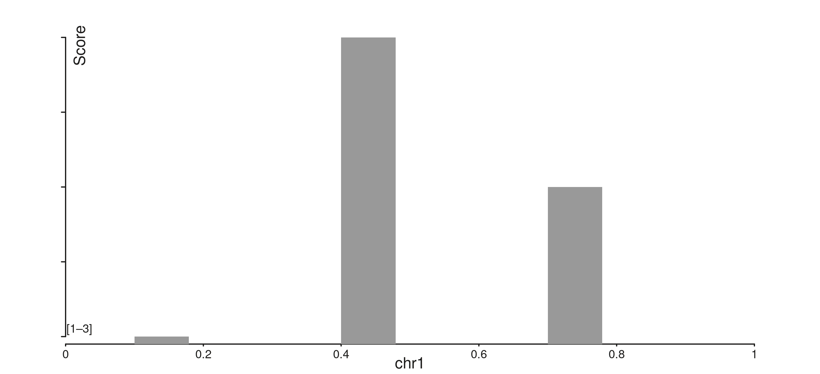

The y-axis here lives entirely inside the panel — the title sits at NPC (0.02, 0.95) (top-left), and a single bracketed range label [lo–hi] sits in the bottom-left corner instead of the per-tick labels.

Composable seq_gene label placement

seq_gene previously placed labels strand-aware to one side of each gene. The new gene.label aes lets you compose label x/y placement independently using c("start"|"end", "top"|"bottom").

gr_genes <- GRanges("chr1",
  IRanges(start = c(100,  400, 1000, 1500),
          end   = c(300,  600, 1200, 1700)),
  gene_id    = c("geneA", "geneA", "geneB", "geneB"),
  gene_name  = c("GeneA", "GeneA", "GeneB", "GeneB"),
  strand_col = c("+", "+", "-", "-"),
  feat_type  = c("exon", "exon", "exon", "exon")
)

win_g <- GRanges("chr1", IRanges(1, 2000))

p <- seq_plot() %+%
  (seq_track(data = gr_genes, windows = win_g) %+%
   seq_gene(
     map(group = gene_id, label = gene_name,
         strand = strand_col, type = feat_type),
     aesthetics = aes(
       gene.label = aes(position = c("start", "top"),
                        color    = "navy",
                        size     = 0.55)
     )
   ))
p$plot()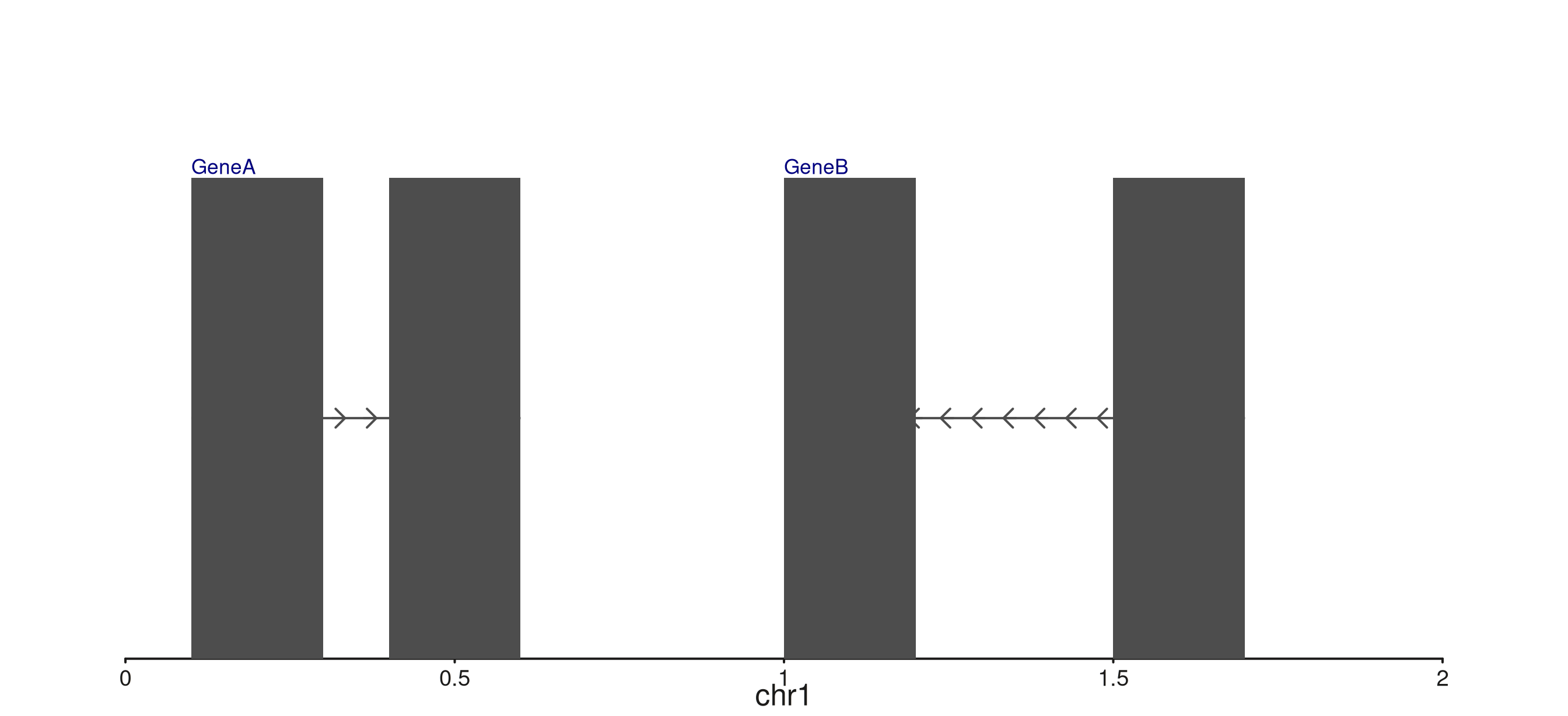

Ideogram scope and style

seq_ideogram(scope = "full") renders the entire chromosome — not just the bands overlapping the current window — and overlays a translucent highlight box marking a sub-range. style = "rounded" adds rounded caps to the two telomere ends.

For axis labels that read chromosome coordinates, give the track the whole chromosome as its windows, then pass highlight_range to mark the sub-range of interest:

cb <- load_cytobands()
chr1_full <- GRanges("chr1", IRanges(1, 248956422))
zoom_in   <- GRanges("chr1", IRanges(1.2e8, 1.6e8))

p <- seq_plot() %+%
  seq_track(windows = zoom_in, height = 1.5) %+%
   seq_ideogram(cb,
                scope           = "full",
                style           = "rounded",
                highlight_range = zoom_in,
                aesthetics = aes(
                  highlight       = aes(fill = "red", alpha = 0.5),
                  telomere.radius = 1
                ))
p$plot()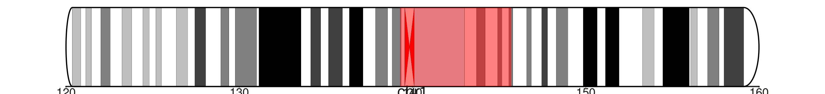

telomere.radius = 1.0 produces a full half-circle cap (cap depth = band height / 2 in inches); smaller values give a shallower curve.

Reference scalebars

seq_scalebar() draws a horizontal length reference at a user-controlled panel position. Useful when the x-axis is hidden but you still want to communicate scale.

win_sb <- GRanges("chr1", IRanges(1, 1e6))

p <- seq_plot() %+%
  (seq_track(
     windows    = win_sb,
     aesthetics = aes("axis.x1.visible" = FALSE)) %+%
   seq_scalebar(length_bp = 1e5,
                hjust     = 0.95,
                vjust     = 0.5,
                bar_lwd   = 1.5))
p$plot()

The label auto-formats from the bp length: 1e5 → "100 kb", 2e6 → "2 Mb", 500 → "500 bp". Override with label = "...".

File connection helpers

open_bigwig(), open_bam(), and open_hic() return lightweight S3 connection objects. Each probes the file header at construction (a few hundred bytes of I/O), records the per-format max_fetch_bp guardrail, and exposes a $fetch(region) method that pulls only the requested genomic span on demand.

bw  <- open_bigwig("path/to/signal.bw")
bw                       # <SeqBigWig>  ...  max_fetch_bp: 50,000,000
sig <- bw$fetch(GRanges("chr1", IRanges(1, 1e6)))   # GRanges of signal

bam <- open_bam("path/to/aln.bam")
bam$fetch(GRanges("chr1", IRanges(20363000, 20370000)))

hic <- open_hic("path/to/contacts.hic", resolution = 25000)
hic$fetch(GRanges("chr1", IRanges(1e7, 1.1e7)))

The guardrail fires before I/O — asking for a span wider than max_fetch_bp raises an informative error rather than silently loading an entire chromosome.

is_seq_file_conn(list())            # FALSE
#> [1] FALSE
is_seq_file_conn("path/to/file.bw") # FALSE
#> [1] FALSE

seq_reads() — IGV-style alignment view

seq_reads() loads alignments from an indexed BAM at construction time, packs them into rows by insert length (or start), and renders chevron polygons (right-pointing for + strand, left for −). Mate pairs are linked by a thin horizontal line by default.

win  <- GRanges("chr1", IRanges(20363000, 20370000))
reads <- seq_reads("path/to/aln.bam", win,
                   sort_by    = "insert_length",
                   link_mates = TRUE)

seq_plot() %+%
  (seq_track(windows = win, height = 4) %+% reads)

Each read becomes one chevron; mate pairs share a single packed row and are connected by their outer extent. The max_width guardrail (default 100 kb) fires before any BAM I/O when a window is too wide.

When a sample BAM is available, the same call renders an IGV-style row- packed view of the underlying alignments:

win_reads <- GRanges("chr20", IRanges(30000000, 30050000))
reads <- seq_reads(demo_bam, win_reads, max_reads = 500)

p <- seq_plot() %+%
  (seq_track(windows = win_reads, height = 4) %+% reads)
p$plot()