SeqPlotR Basics: Composite Elements

This vignette walks through the composite elements in SeqPlotR using toy GRanges data. Each section builds a small synthetic dataset and renders the element via the seq_plot() %+% seq_track() %+% <element> pipeline.

Coordinate conventions

SeqPlotR automatically selects the x-axis unit from the narrowest window in each track:

Narrowest window width	Displayed unit	scale_factor
≥ 1 Mb (1,000,000 bp)	Mb	1e-6
≥ 100 bp	kb	1e-3
< 100 bp	bp	1

All windows in a track share the same unit so axis break intervals are consistent across panels. Override per-track with seq_track(window_scale = ...), or per-window by setting mcols(windows)$scale directly (highest priority). The examples below use 2 Mb windows, which auto-infer the Mb unit.

library(SeqPlotR)
#> 
#> Attaching package: 'SeqPlotR'
#> The following object is masked from 'package:base':
#> 
#>     %||%
library(GenomicRanges)
#> Loading required package: stats4
#> Loading required package: BiocGenerics
#> Loading required package: generics
#> 
#> Attaching package: 'generics'
#> The following objects are masked from 'package:base':
#> 
#>     as.difftime, as.factor, as.ordered, intersect, is.element, setdiff,
#>     setequal, union
#> 
#> Attaching package: 'BiocGenerics'
#> The following objects are masked from 'package:stats':
#> 
#>     IQR, mad, sd, var, xtabs
#> The following objects are masked from 'package:base':
#> 
#>     anyDuplicated, aperm, append, as.data.frame, basename, cbind,
#>     colnames, dirname, do.call, duplicated, eval, evalq, Filter, Find,
#>     get, grep, grepl, is.unsorted, lapply, Map, mapply, match, mget,
#>     order, paste, pmax, pmax.int, pmin, pmin.int, Position, rank,
#>     rbind, Reduce, rownames, sapply, saveRDS, table, tapply, unique,
#>     unsplit, which.max, which.min
#> Loading required package: S4Vectors
#> 
#> Attaching package: 'S4Vectors'
#> The following object is masked from 'package:utils':
#> 
#>     findMatches
#> The following objects are masked from 'package:base':
#> 
#>     expand.grid, I, unname
#> Loading required package: IRanges
#> Loading required package: Seqinfo

# A single 2-Mb window on chr1 → axis labels read as 1.0, 1.5, 2.0 Mb.
win <- GRanges("chr1", IRanges(1e6, 3e6))

Tracks, windows, and margins

Every track is allocated a rectangular cell in the page layout and partitioned into five nested zones, two at the track level and three at the window level:

• Track outer margin — outermost band on the track cell. Axis titles (taken from the track mapping) are drawn here. seq_track(track_outer_margin = ...). Default 0.02.
• Track inner margin — separates the title band from the window row. seq_track(track_inner_margin = ...). Default 0.02.
• Window outer margin — per-window spacer inside the track plot region. seq_track(window_outer_margin = ...). Default 0.
• Window inner margin — per-window band holding axis lines, ticks, and tick labels. seq_track(window_inner_margin = ...). Default 0.02.
• Plot area — what remains per window. Elements render here; panel$inner carries these coordinates.

Axis lines sit at the boundary between the plot area and the window inner margin. The gap between adjacent windows is the plot- or track-level aes("window.gap.width" = ...) (default 0.01); the gap between tracks is the plot-level trackGaps (default 0.01). The old seq_track(window_margin = ...) constructor argument is deprecated — see Window gap width below.

The schematic below lays out two tracks × two windows using nothing but SeqPlotR, with each zone coloured via the plot-level trackBackground, trackInnerBackground, windowBoxBackground, windowInnerBackground, and windowBackground aesthetics. seq_text places a label in each plot area.

# Two windows (2 Mb and 1.5 Mb wide).
schematic_win <- GRanges(
  "chr1", IRanges(start = c(1e6, 5e6), end = c(3e6, 6.5e6)))

# One label centred inside each window for each track.
mk_labels <- function(track_name) {
  GRanges(
    "chr1", IRanges(start = c(2e6, 5.75e6), width = 1),
    label = paste0(track_name, "\nWindow ", c(1, 2))
  )
}
lbl_A <- mk_labels("Track A")
lbl_B <- mk_labels("Track B")

# Zone colors via plot-level aesthetics; axes turned off so the five
# nested rectangles are visible without interference.
schematic_aes <- aes(
  trackBackground        = "#F89A8A",  # track outer margin
  trackBorder            = "grey30",
  trackInnerBackground   = "#ECCB60",  # track inner margin
  trackInnerBorder       = "grey30",
  windowBoxBackground    = "#A699D0",  # window outer margin
  windowBoxBorder        = "grey30",
  windowInnerBackground  = "#BEC97E",  # window inner margin
  windowInnerBorder      = "grey30",
  windowBackground       = "#92BFDB",  # plot area
  windowBorder           = "grey30",
  xAxisLine = FALSE, xAxisTicks = FALSE, xAxisLabels = FALSE,
  xAxisTitle = FALSE,
  yAxisLine = FALSE, yAxisTicks = FALSE, yAxisLabels = FALSE,
  yAxisTitle = FALSE,
  trackGaps = 0.04,
  "window.gap.width" = 0.03
)

seq_plot(aesthetics = schematic_aes) %|%
  seq_track(track_id = "A",
            data = lbl_A,
            mapping = map(x = start, label = label),
            windows = schematic_win,
            track_outer_margin  = 0.035,
            track_inner_margin  = 0.025,
            window_outer_margin = 0.025,
            window_inner_margin = 0.035) %+%
  seq_text(aesthetics = aes(fontsize = 12, color = "#1C1B1A")) %__%
  seq_track(track_id = "B",
            data = lbl_B,
            mapping = map(x = start, label = label),
            windows = schematic_win,
            track_outer_margin  = 0.035,
            track_inner_margin  = 0.025,
            window_outer_margin = 0.025,
            window_inner_margin = 0.035) %+%
  seq_text(aesthetics = aes(fontsize = 12, color = "#1C1B1A")) -> p
p$plot()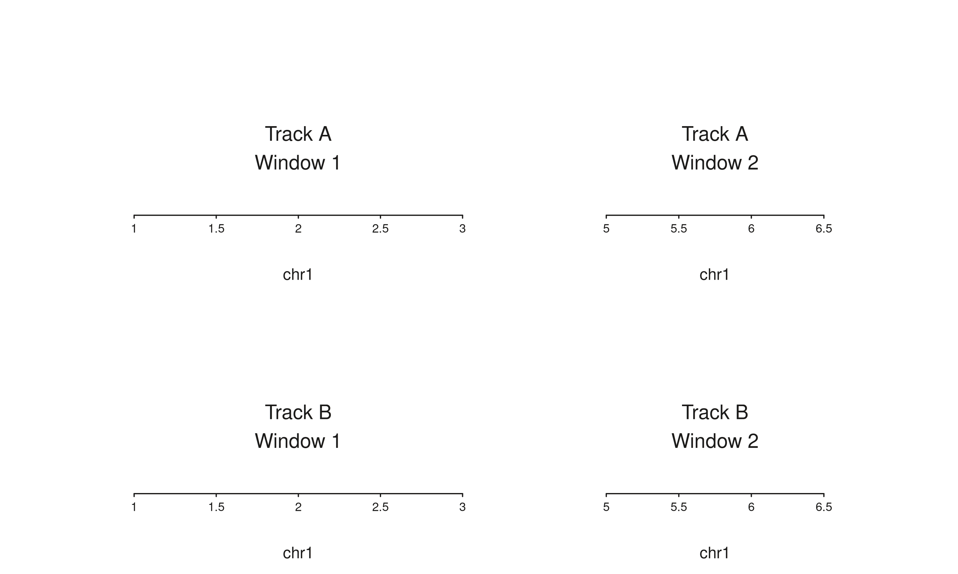

Reading the schematic, from outside to inside on each track:

• Pink — track outer margin (axis titles live here).
• Yellow — track inner margin.
• Purple — window outer margin (per-window spacer).
• Green — window inner margin (axis lines, ticks, tick labels live here).
• Blue — plot area, where elements render.
• The vertical green/blue split inside a track is the window margin between the two windows.
• The horizontal gap between the two tracks is the track gap.

The next chunk shows the same layout with real elements and axes on. Axis titles appear in the track outer margin, pulling their text directly from the track mapping (the x title is start, the y titles are score and impact).

trkA_gr <- GRanges("chr1",
  IRanges(start = c(1.2e6, 1.8e6, 2.4e6, 5.2e6, 5.7e6, 6.2e6), width = 1e5),
  score = c(0.3, 0.7, 0.5, 0.6, 0.4, 0.8))

trkB_gr <- GRanges("chr1",
  IRanges(start = c(1.3e6, 2.0e6, 2.7e6, 5.3e6, 5.9e6, 6.3e6), width = 1),
  impact = c(0.5, 0.9, 0.4, 0.7, 0.3, 0.6))

real_aes <- aes(
  trackBackground      = "#FCEBEA",
  trackInnerBackground = "#FAF5DC",
  "window.gap.width"   = 0.02
)

seq_plot(aesthetics = real_aes) %|%
  seq_track(track_id = "Track A",
            data = trkA_gr,
            mapping = map(x = start, y = score),
            windows = schematic_win,
            track_outer_margin = 0.03,
            window_inner_margin = 0.04) %+%
  seq_bar(aesthetics = aes(fill = "#4385BE")) %__%
  seq_track(track_id = "Track B",
            data = trkB_gr,
            mapping = map(x = start, y = impact),
            windows = schematic_win,
            track_outer_margin = 0.03,
            window_inner_margin = 0.04) %+%
  seq_lollipop(aesthetics = aes(color = "#AF3029", linewidth = 1.2)) -> p
p$plot()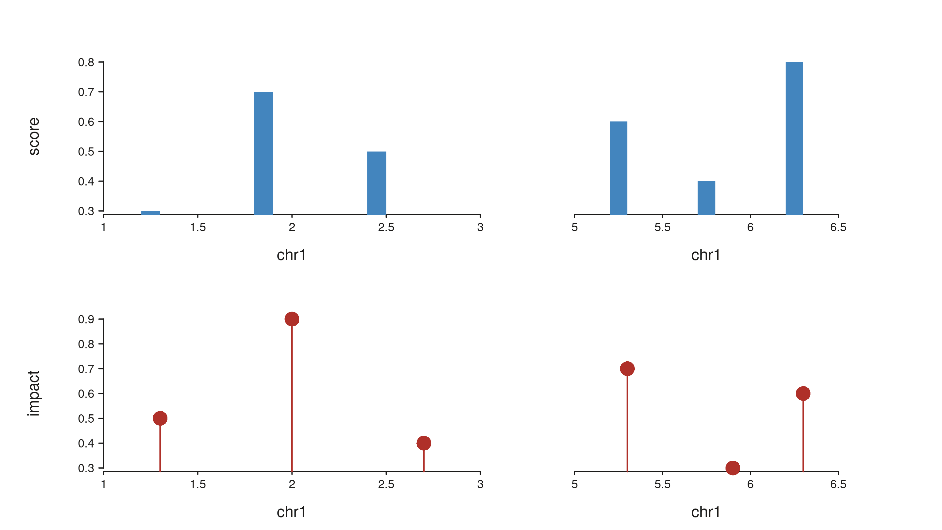

Window gap width

aes("window.gap.width" = <npc>) controls the horizontal gap between adjacent windows within a track. Set it on seq_plot() to apply across every track, or on a specific seq_track() to override the plot-level value for that track only. Default is 0.01.

gap_win <- GRanges(
  "chr1",
  IRanges(start = c(1, 1e6 + 1, 2e6 + 1), width = 1e6)
)
gap_lbl <- function(track_name) {
  GRanges(
    "chr1",
    IRanges(start = c(5e5, 1.5e6, 2.5e6), width = 1),
    label = paste0(track_name, "\nW", c(1, 2, 3))
  )
}

# Three tracks, three gap widths: collapsed, default, generous.
seq_plot(aesthetics = aes(
    windowBackground = "#92BFDB", windowBorder = "grey30",
    xAxisLine = FALSE, xAxisTicks = FALSE, xAxisLabels = FALSE,
    xAxisTitle = FALSE, yAxisLine = FALSE, yAxisTicks = FALSE,
    yAxisLabels = FALSE, yAxisTitle = FALSE,
    "window.gap.width" = 0   # plot-level default for all tracks
  )) %|%
  seq_track(track_id = "Collapsed (0)",
            data = gap_lbl("Collapsed"),
            mapping = map(x = start, label = label),
            windows = gap_win) %+%
  seq_text(aesthetics = aes(fontsize = 11)) %__%
  seq_track(track_id = "Default (0.01)",
            data = gap_lbl("Default"),
            mapping = map(x = start, label = label),
            windows = gap_win,
            aesthetics = aes("window.gap.width" = 0.01)) %+%
  seq_text(aesthetics = aes(fontsize = 11)) %__%
  seq_track(track_id = "Generous (0.05)",
            data = gap_lbl("Generous"),
            mapping = map(x = start, label = label),
            windows = gap_win,
            aesthetics = aes("window.gap.width" = 0.05)) %+%
  seq_text(aesthetics = aes(fontsize = 11)) -> p
p$plot()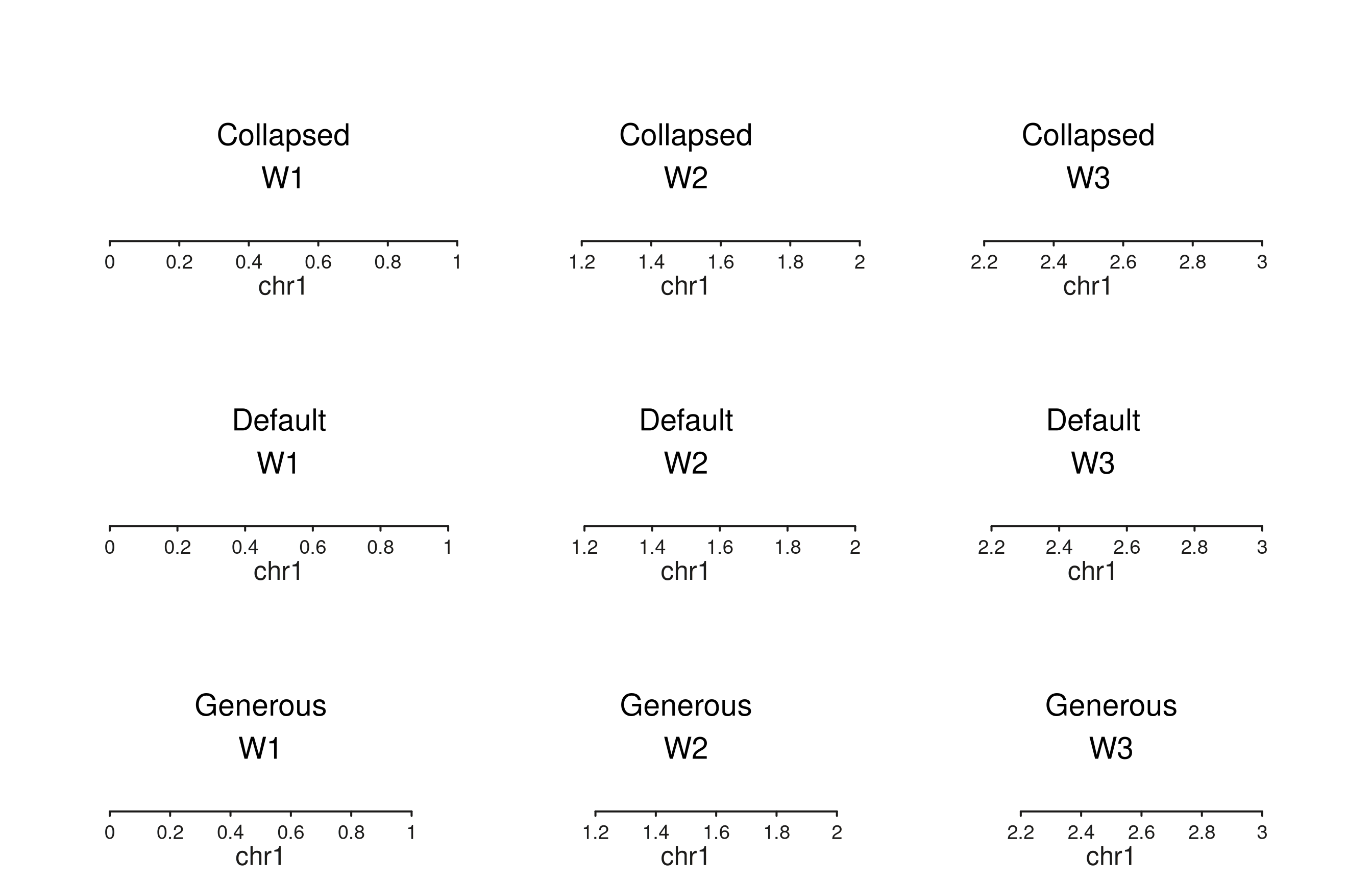

The legacy seq_track(window_margin = ...) constructor argument is deprecated and emits a warning when used; switch to aes("window.gap.width" = ...). The older aes(window_gaps = ...) key still works as an alias but window.gap.width takes priority when both are set.

Margin recipes

The five zones are independent knobs. The examples below share a single small dataset and vary only the margin arguments so the effect of each one is visible.

recipe_win <- GRanges("chr1", IRanges(1e6, 3e6))
recipe_gr  <- GRanges(
  "chr1",
  IRanges(start = seq(1.1e6, 2.9e6, by = 2e5), width = 8e4),
  score = runif(10, 0.2, 1.0)
)

Minimal: drop the axis titles and the track outer margin — the plot fills the full track cell.

seq_plot(aesthetics = aes(xAxisTitle = FALSE, yAxisTitle = FALSE)) %|%
  seq_track(data = recipe_gr,
            mapping = map(x = start, y = score),
            windows = recipe_win,
            track_outer_margin = 0,
            window_inner_margin = 0.02) %+%
  seq_bar(aesthetics = aes(fill = "#4385BE")) -> p
p$plot()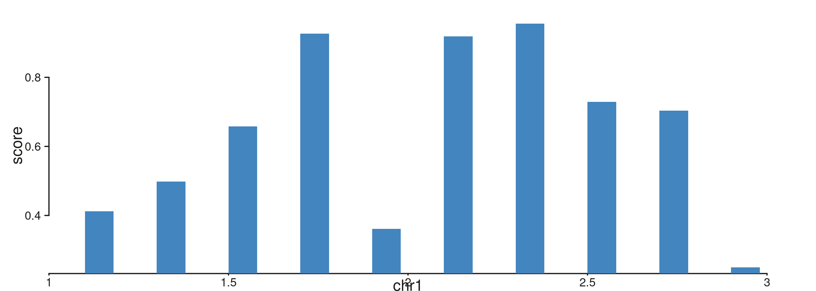

Room for titles and labels: widen both track and window margins. The axis titles (start, score) auto-populate from the mapping.

seq_plot() %|%
  seq_track(data = recipe_gr,
            mapping = map(x = start, y = score),
            windows = recipe_win,
            track_outer_margin = c(0.05, 0.05, 0.02, 0.02),
            window_inner_margin = 0.06) %+%
  seq_bar(aesthetics = aes(fill = "#4385BE")) -> p
p$plot()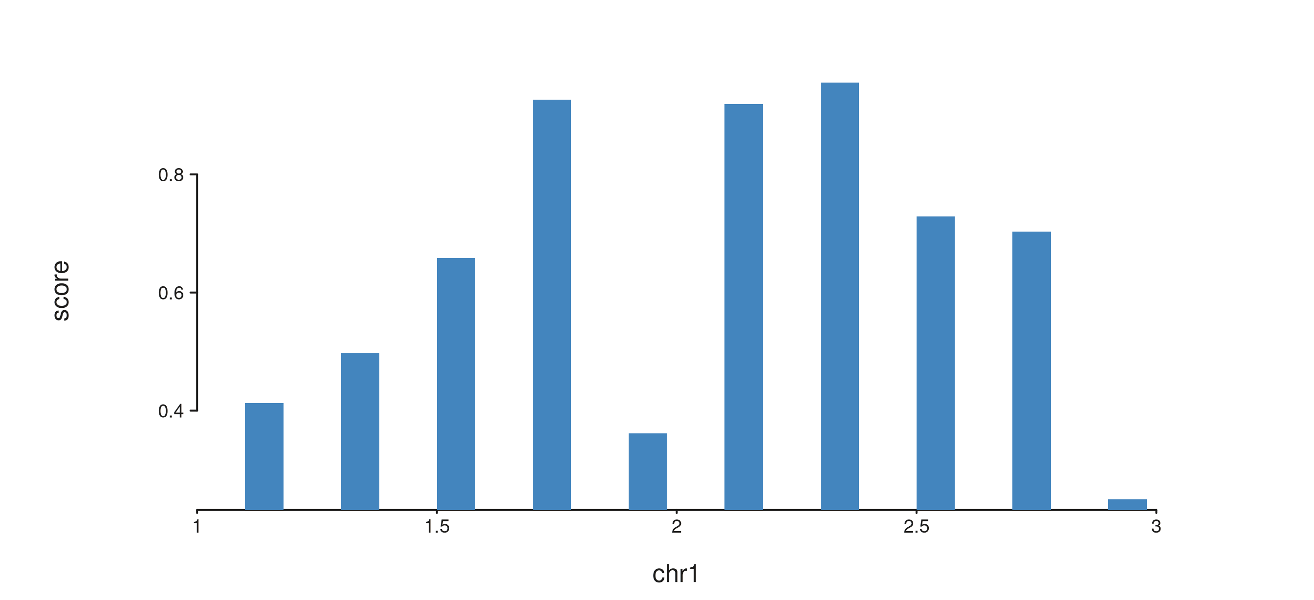

Asymmetric margins: the length-4 form uses base-R par(mar = c(bottom, left, top, right)) order. Below the x-axis title gets a wider bottom band; the top edge stays flush.

seq_plot() %|%
  seq_track(data = recipe_gr,
            mapping = map(x = start, y = score),
            windows = recipe_win,
            track_outer_margin = c(0.06, 0.06, 0, 0),
            track_inner_margin = 0.015,
            window_inner_margin = 0.04) %+%
  seq_bar(aesthetics = aes(fill = "#4385BE")) -> p
p$plot()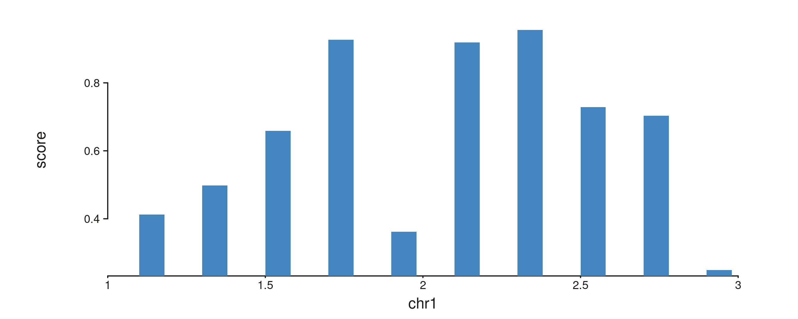

Window inner vs window outer margin: turn on windowBoxBackground and windowInnerBackground to see the two per-window bands. The window outer margin (purple) is an optional spacer; the window inner margin (green) is where ticks and labels sit.

seq_plot(aesthetics = aes(
    windowBoxBackground   = "#C4B9E0",
    windowInnerBackground = "#BEC97E"
  )) %|%
  seq_track(data = recipe_gr,
            mapping = map(x = start, y = score),
            windows = recipe_win,
            track_outer_margin  = 0.03,
            track_inner_margin  = 0.01,
            window_outer_margin = 0.02,
            window_inner_margin = 0.05) %+%
  seq_bar(aesthetics = aes(fill = "#4385BE")) -> p
p$plot()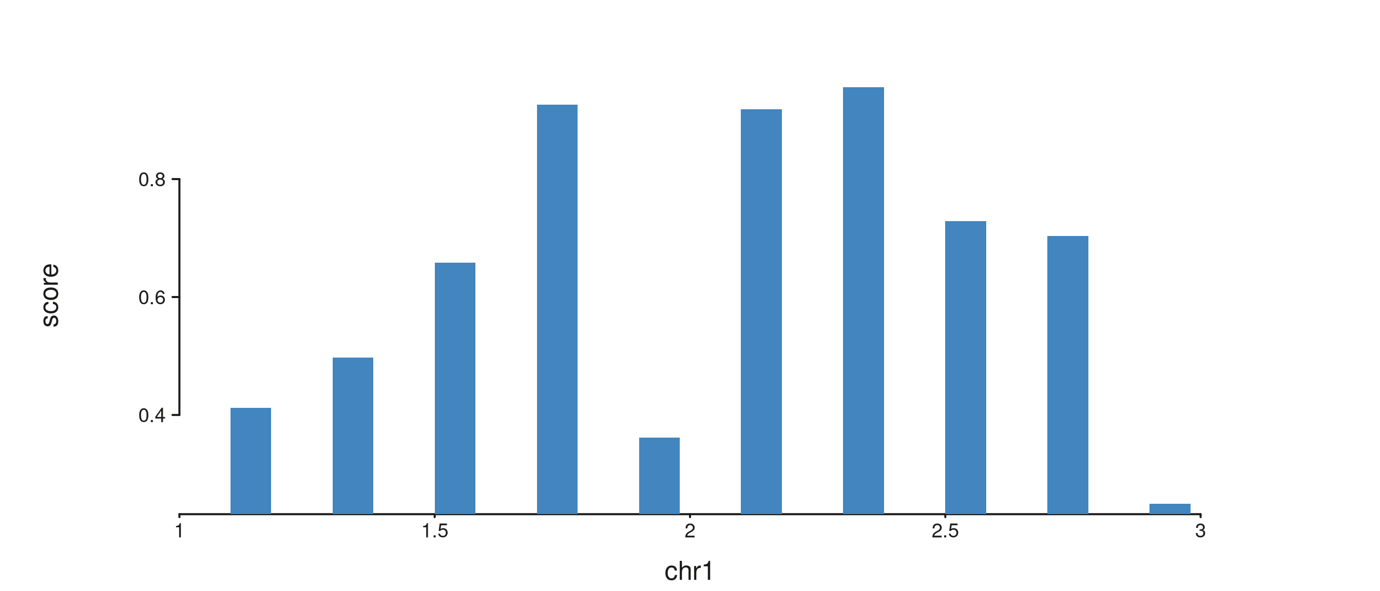

Track and window sizing

Relative sizing is controlled by three arguments: track_width (within a row), track_height (across rows), and the scale mcols column on the windows GRanges (within a track’s plot region).

Unequal track widths on one row. Track A is 3× wider than B.

win_small <- GRanges("chr1", IRanges(1e6, 3e6))
gr_small  <- GRanges("chr1",
  IRanges(start = seq(1.1e6, 2.9e6, by = 2e5), width = 8e4),
  score = runif(10, 0.2, 1.0))

seq_plot() %|%
  seq_track(track_id = "A",
            data = gr_small,
            mapping = map(x = start, y = score),
            windows = win_small,
            track_width = 3) %+%
  seq_bar(aesthetics = aes(fill = "#4385BE")) %|%
  seq_track(track_id = "B",
            data = gr_small,
            mapping = map(x = start, y = score),
            windows = win_small,
            track_width = 1) %+%
  seq_lollipop(aesthetics = aes(color = "#AF3029")) -> p
p$plot()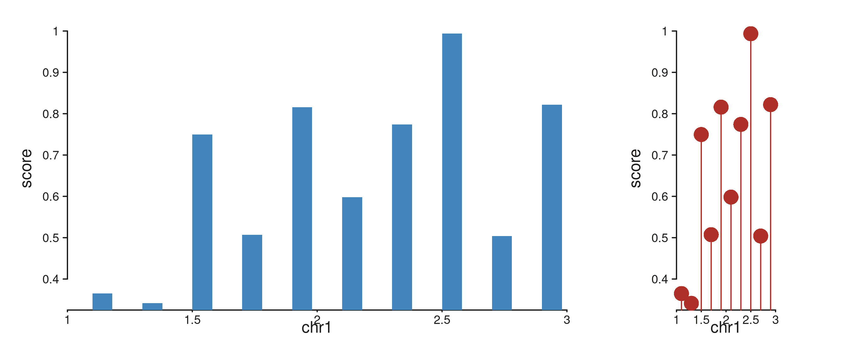

Unequal track heights on stacked rows. A points track twice as tall as the bar track below it.

xs_sig <- seq(1.05e6, 2.95e6, length.out = 40)
sig_gr <- GRanges("chr1", IRanges(start = xs_sig, width = 1),
                  score = sin((xs_sig - 1e6) / 3e5) * 0.4 + 0.5)

seq_plot() %|%
  seq_track(track_id = "Signal",
            data = sig_gr,
            mapping = map(x = start, y = score),
            windows = win_small,
            track_height = 2) %+%
  seq_line(aesthetics = aes(color = "#4385BE", linewidth = 1.5)) %__%
  seq_track(track_id = "Bars",
            data = gr_small,
            mapping = map(x = start, y = score),
            windows = win_small,
            track_height = 1) %+%
  seq_bar(aesthetics = aes(fill = "#8B7EC8")) -> p
p$plot()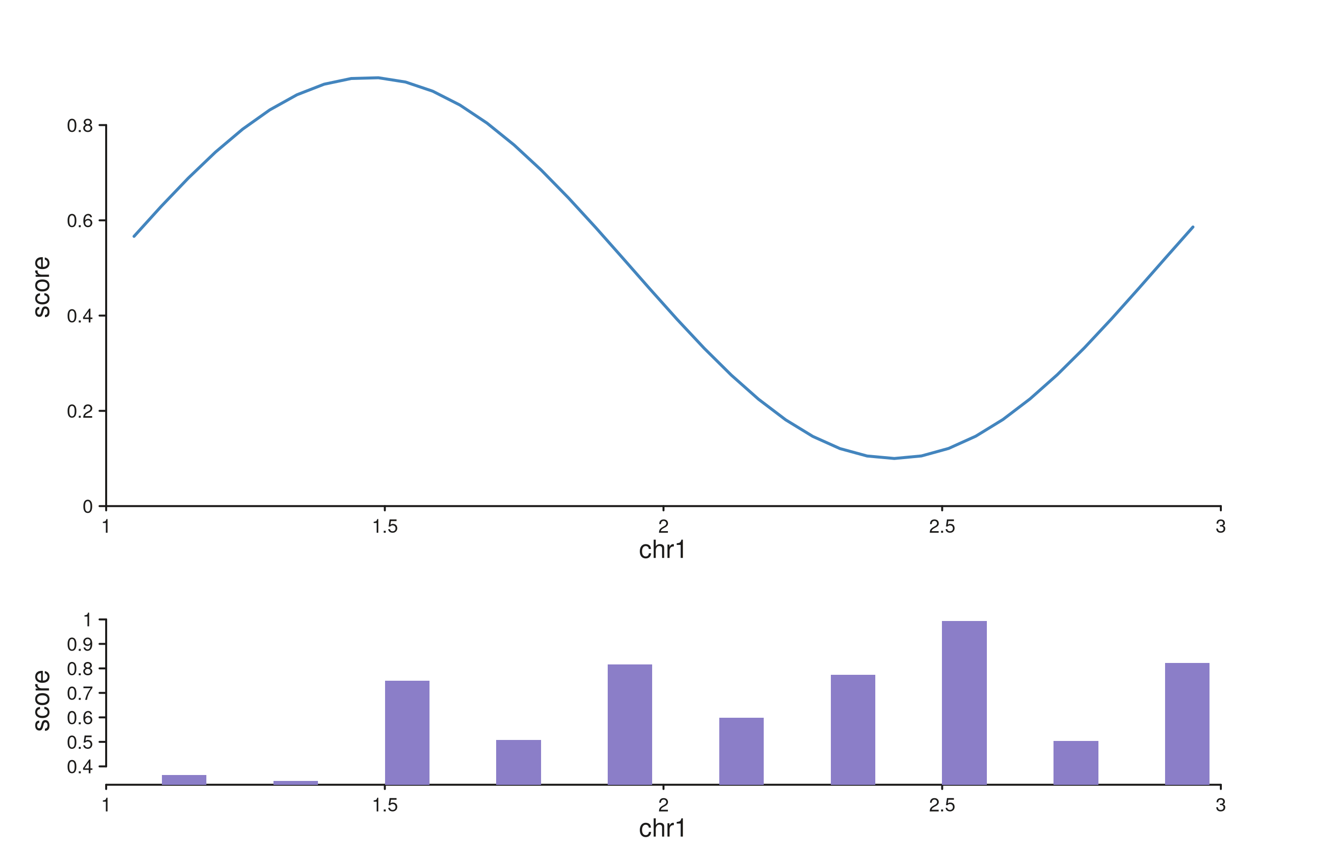

Per-window scale factor. Within a multi-window track, windows are sized by width(windows) * mcols(windows)$scale. Defaults to the auto-inferred scale for all windows. Setting one window’s scale to 0 shrinks it to nothing; setting distinct scales compresses or expands individual windows relative to others.

# Two windows of equal genomic width, but the second rendered at
# 2× the first's relative width.
scaled_win <- GRanges(
  "chr1", IRanges(start = c(1e6, 5e6), end = c(3e6, 7e6)))
S4Vectors::mcols(scaled_win)$scale <- c(1e-6, 2e-6)

scaled_gr <- GRanges("chr1",
  IRanges(start = c(seq(1.2e6, 2.8e6, length.out = 5),
                    seq(5.2e6, 6.8e6, length.out = 5)),
          width = 1e5),
  score = runif(10, 0.2, 1.0))

seq_plot() %|%
  seq_track(data = scaled_gr,
            mapping = map(x = start, y = score),
            windows = scaled_win) %+%
  seq_bar(aesthetics = aes(fill = "#4385BE")) -> p
p$plot()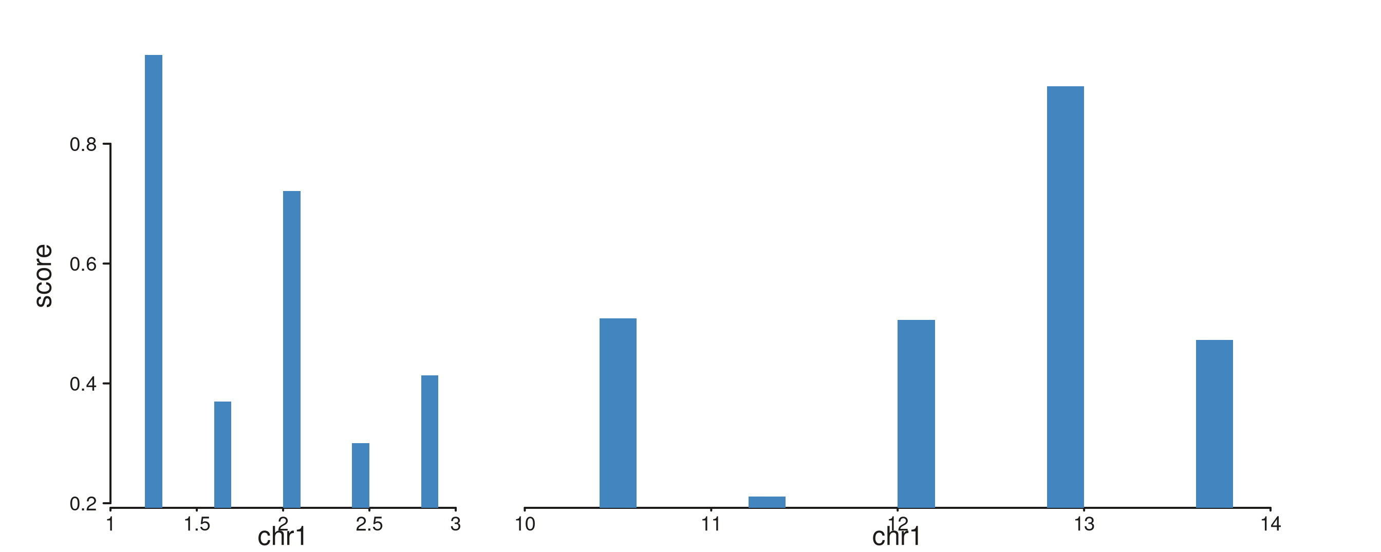

Track-level unit override with window_scale. Pass window_scale on seq_track to force a fixed scale factor for all windows, or a positional vector to set each window independently. window_scale overrides the auto-inferred unit but is overridden by any mcols(windows)$scale already present. Length-1 applies to all windows; any other mismatched length triggers a warning and recycles.

# Two 5 Mb windows — auto-inference gives Mb, but we force kb.
mb_win <- GRanges("chr1", IRanges(start = c(1e6, 1e7 + 1), width = 5e6))
mb_gr  <- GRanges("chr1",
  IRanges(start = c(seq(1.2e6, 5.8e6, length.out = 5),
                    seq(1.02e7, 1.58e7, length.out = 5)),
          width = 2e5),
  score = runif(10, 0.2, 1.0))

seq_plot() %|%
  seq_track(data = mb_gr,
            mapping = map(x = start, y = score),
            windows = mb_win,
            window_scale = 1e-3) %+%
  seq_bar(aesthetics = aes(fill = "#4385BE")) -> p
p$plot()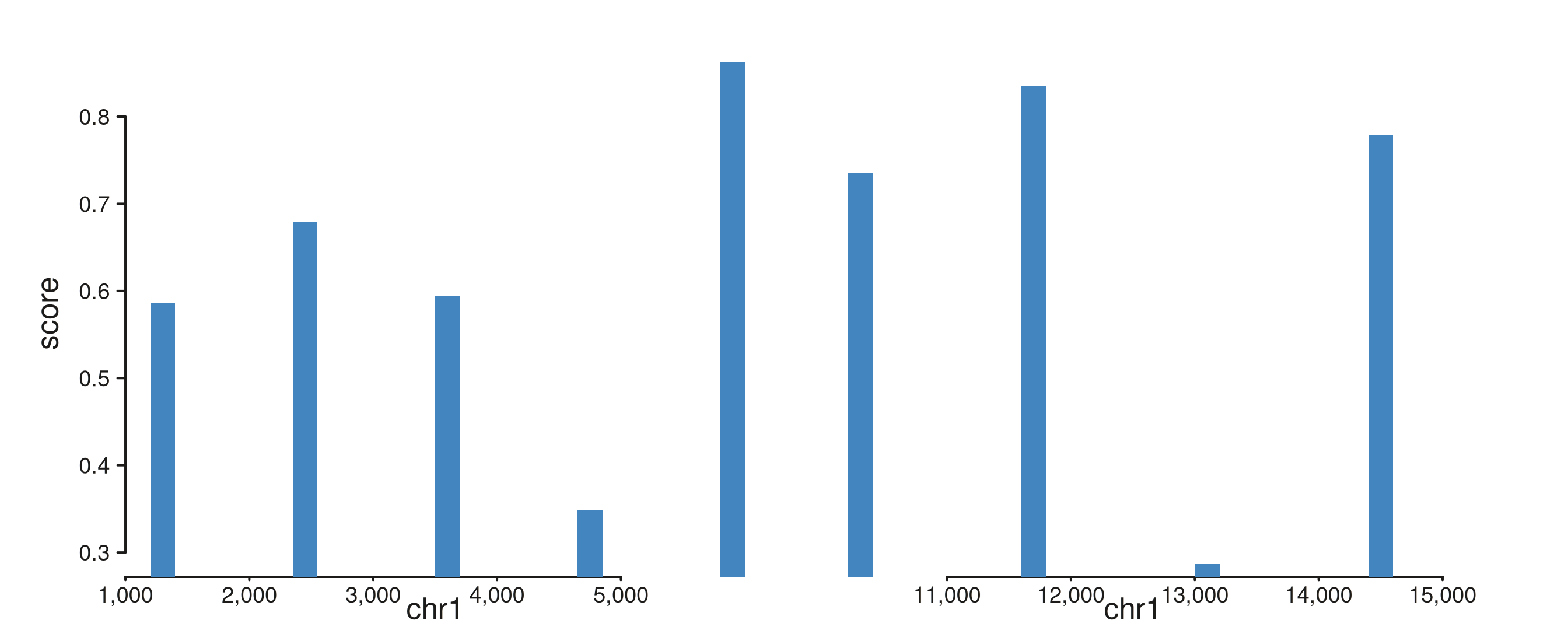

seq_bar — simple bars

One filled rectangle per interval. With no group mapping, each bar’s height is its mapped y value.

bar_gr <- GRanges(
  "chr1",
  IRanges(start = seq(1.1e6, 2.9e6, by = 2e5), width = 8e4),
  score = runif(10, 0.2, 1.0)
)

seq_plot() %|%
  seq_track(data = bar_gr,
            mapping = map(x = start, y = score),
            windows = win) %+%
  seq_bar() -> p
p$plot()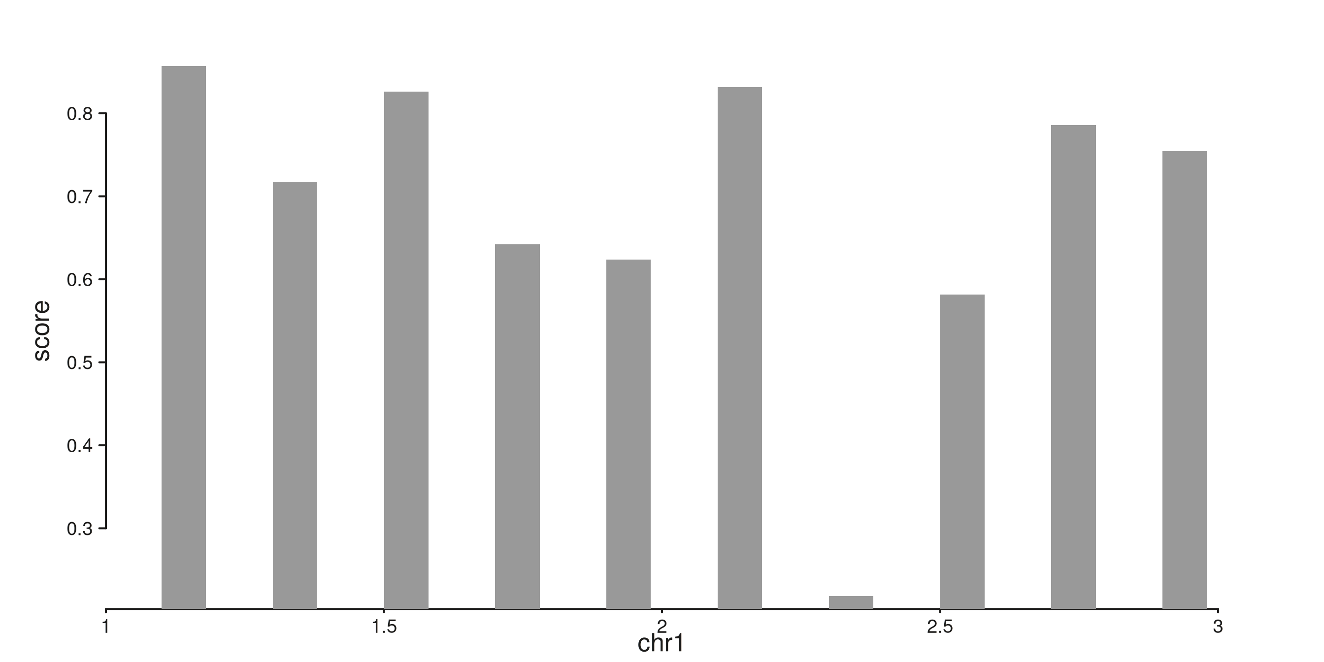

Stacked bars

Supplying a group mapping causes bars at identical x positions to stack. Colors are drawn from the Flexoki palette keyed on group level.

stack_gr <- GRanges(
  "chr1",
  IRanges(start = rep(seq(1.2e6, 2.8e6, by = 2e5), each = 3), width = 5e4),
  value    = runif(27, 0.1, 0.5),
  category = rep(c("A", "B", "C"), times = 9)
)

seq_plot() %|%
  seq_track(data = stack_gr,
            mapping = map(x = start, y = value, group = category),
            windows = win) %+%
  seq_bar() -> p
p$plot()
#> 8 out-of-bounds data points excluded! (seq_bar)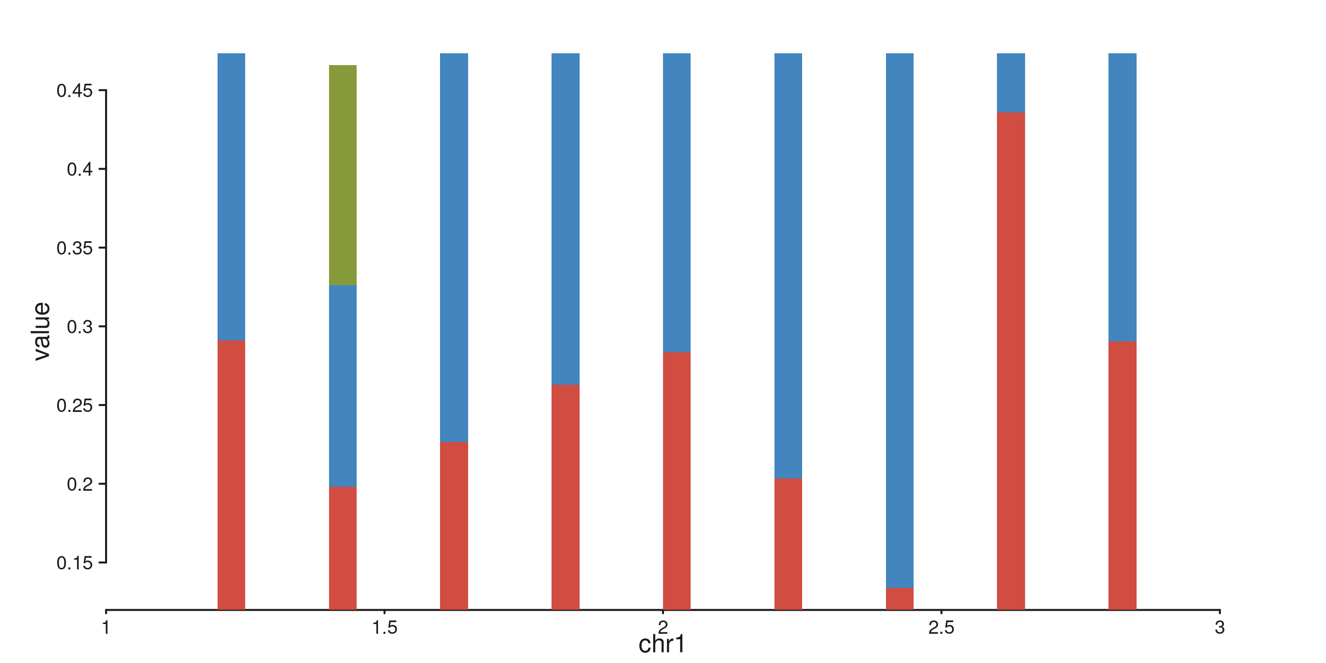

seq_ribbon — filled band between two y series

Requires y_min and y_max mappings. Useful for confidence bands.

xs <- seq(1.05e6, 2.95e6, length.out = 50)
mu <- sin((xs - 1e6) / 3e5) * 0.3 + 0.5
band <- 0.15

ribbon_gr <- GRanges(
  "chr1", IRanges(start = xs, width = 1),
  mean = mu,
  lo   = mu - band,
  hi   = mu + band
)

seq_plot() %|%
  seq_track(data = ribbon_gr,
            mapping = map(x = start, y_min = lo, y_max = hi),
            windows = win) %+%
  seq_ribbon(aesthetics = aes(fill = "#4385BE", alpha = 0.5)) -> p
p$plot()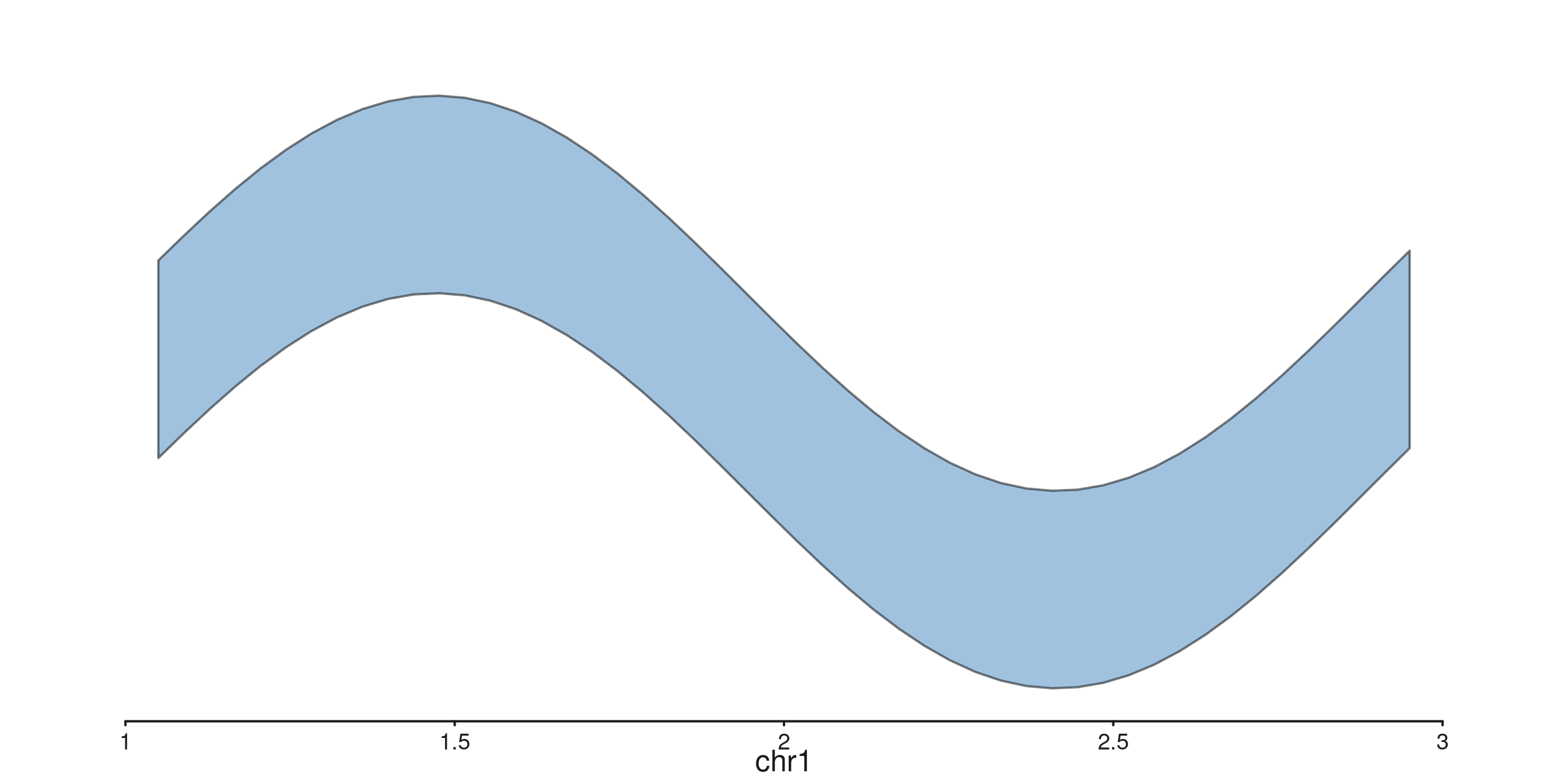

seq_density — kernel density estimate

Computes stats::density() on the mapped y and renders the distribution as a filled area. The density evaluation axis runs horizontally, mapped through the track’s yscale.

dens_gr <- GRanges(
  "chr1", IRanges(start = seq(1e6, 3e6, length.out = 200), width = 1),
  score = c(rnorm(120, mean = 0.3, sd = 0.05),
            rnorm(80,  mean = 0.7, sd = 0.08))
)

seq_plot() %|%
  seq_track(data = dens_gr,
            mapping = map(x = start, y = score),
            windows = win) %+%
  seq_density(aesthetics = aes(fill = "#879A39", alpha = 0.7)) -> p
p$plot()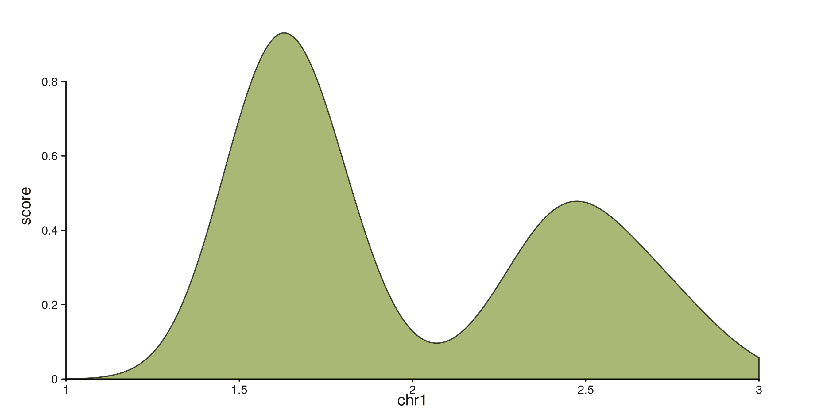

seq_tile — rectangles per interval

Unrotated (default): one rectangle per observation

tile_gr <- GRanges(
  "chr1",
  IRanges(start = seq(1.1e6, 2.9e6, by = 1e5), width = 8e4),
  fill_col = sample(flexoki_palette(5), 19, replace = TRUE)
)

seq_plot() %|%
  seq_track(data = tile_gr,
            mapping = map(x = start, fill = fill_col),
            windows = win) %+%
  seq_tile(aesthetics = aes(rotate = FALSE)) -> p
p$plot()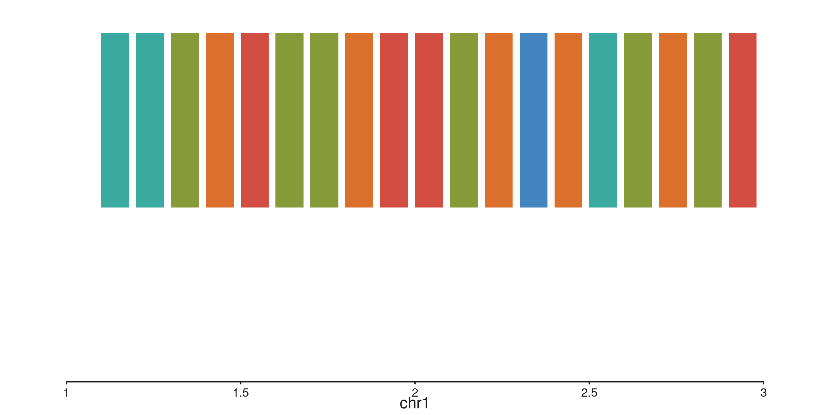

seq_lollipop — stem + point

Vertical stem from baseline (default 0) to y, with a point at y. Good for sparse, discrete events (e.g. mutation calls).

lp_gr <- GRanges(
  "chr1",
  IRanges(start = sample(seq(1.05e6, 2.95e6, by = 1e4), 15), width = 1),
  impact = runif(15, 0.2, 1.0)
)

seq_plot() %|%
  seq_track(data = lp_gr,
            mapping = map(x = start, y = impact),
            windows = win) %+%
  seq_lollipop(aesthetics = aes(color = "#AF3029", linewidth = 1.2)) -> p
p$plot()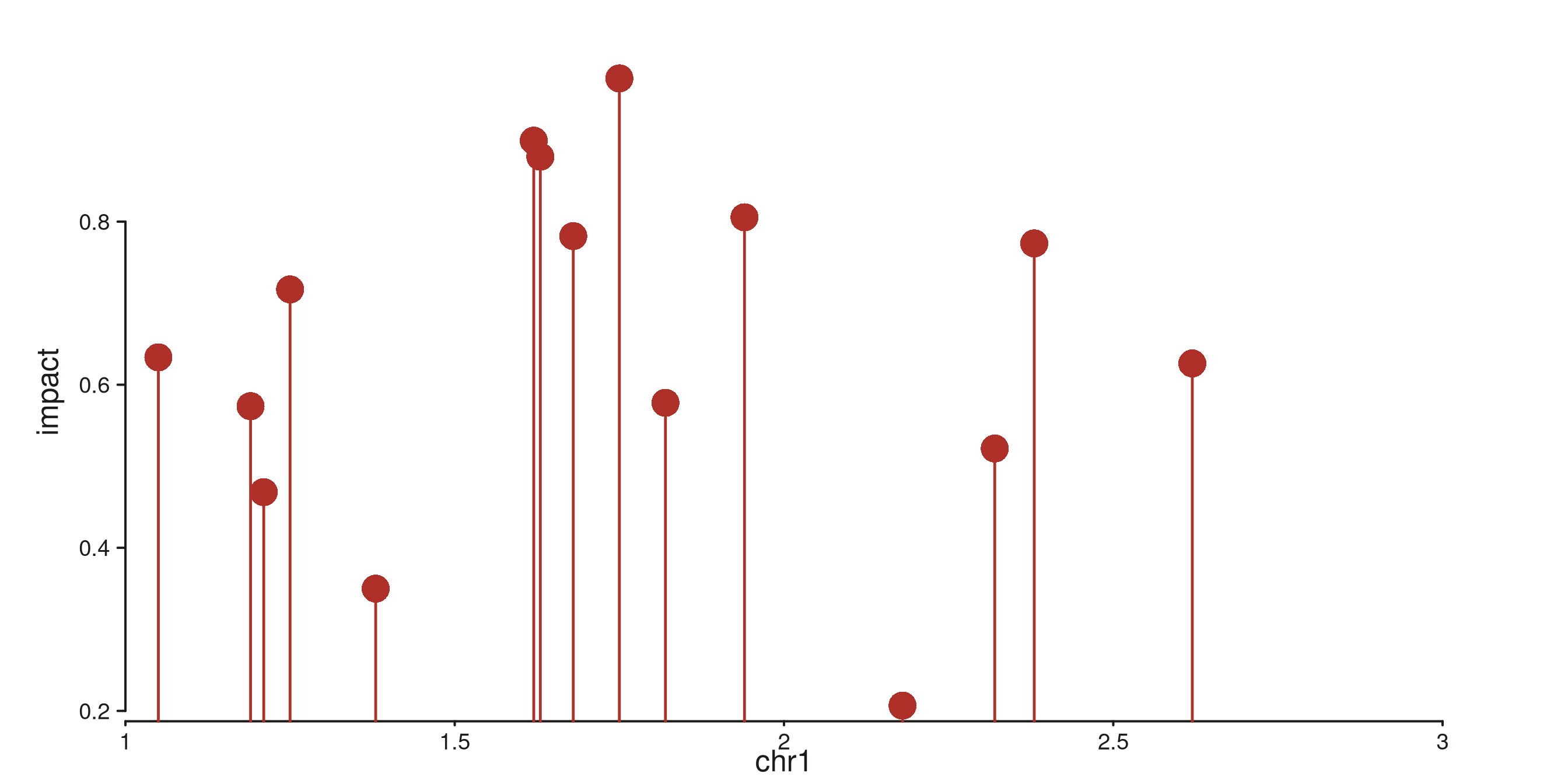

seq_gene — format-agnostic gene models

All column references come through map(): group joins features into one gene, strand orients the arrows, type distinguishes exons from UTRs, label places the gene name, and color tints each gene.

gene_gr <- GRanges(
  "chr1",
  IRanges(
    start = c(1.10e6, 1.20e6, 1.35e6, 1.50e6, 1.58e6,
              1.90e6, 2.05e6, 2.18e6, 2.30e6,
              2.55e6, 2.68e6, 2.80e6),
    width = c( 3e4,  6e4,  4e4,  5e4,  2e4,
               4e4,  8e4,  5e4,  3e4,
               6e4,  3e4,  5e4)
  ),
  gene_id   = c("A","A","A","A","A",
                "B","B","B","B",
                "C","C","C"),
  gene_name = c("TP53","TP53","TP53","TP53","TP53",
                "MYC","MYC","MYC","MYC",
                "BRCA1","BRCA1","BRCA1"),
  strand_col = c("+","+","+","+","+",
                 "-","-","-","-",
                 "+","+","+"),
  feature = c("UTR","exon","exon","exon","UTR",
              "UTR","exon","exon","UTR",
              "exon","exon","exon"),
  color = c(rep("#205EA6", 5),
            rep("#AF3029", 4),
            rep("#66800B", 3))
)

seq_plot() %|%
  seq_track(data = gene_gr,
            mapping = map(group  = gene_id,
                          type   = feature,
                          strand = strand_col,
                          label  = gene_name,
                          color  = color),
            windows = win) %+%
  seq_gene(map(group  = gene_id,
               type   = feature,
               strand = strand_col,
               label  = gene_name,
               color  = color)) -> p
p$plot()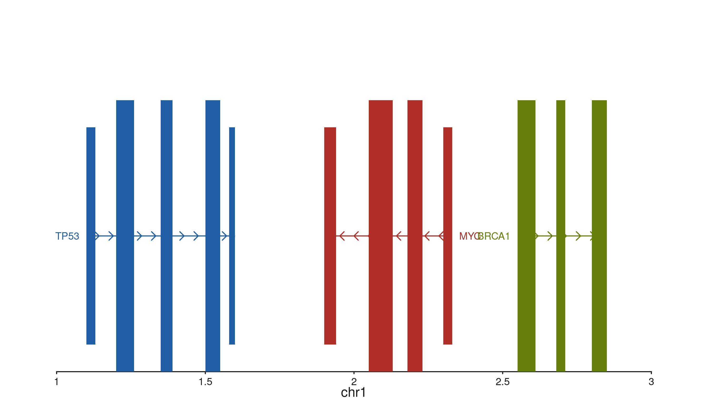

Multi-region windows

A single windows GRanges may contain several ranges. Each window becomes its own panel within the same track, with relative widths set by width(windows). The same mapping resolves against every window independently, and per-panel x-scales reflect the local coordinates.

multi_win <- GRanges(
  "chr1",
  IRanges(start = c(1.0e6, 5.0e6), end = c(3.0e6, 6.5e6))
)

starts_A <- seq(1.1e6, 2.9e6, length.out = 10)  # 10 in window 1
starts_B <- seq(5.1e6, 6.4e6, length.out = 10)  # 10 in window 2
multi_gr <- GRanges(
  "chr1",
  IRanges(start = c(starts_A, starts_B), width = 5e4),
  score  = runif(20, 0.2, 1.0),
  region = rep(c("Region A", "Region B"), times = c(10, 10))
)

seq_plot() %|%
  seq_track(data = multi_gr,
            mapping = map(x = start, y = score, group = region),
            windows = multi_win) %+%
  seq_bar() -> p
p$plot()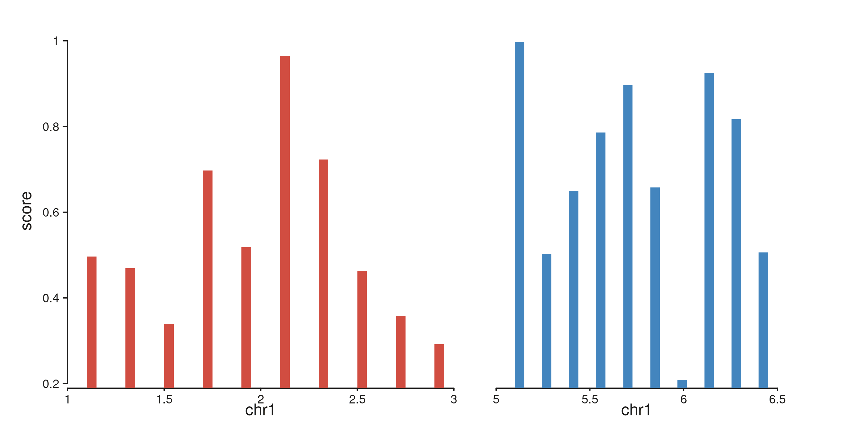

Flipping the axes: genomic on x vs. genomic on y

By default every seq_track runs genomic x along its width and lets elements choose the y-axis scale from their data. Pass scale_y = seq_scale_genomic(...) to flip the track so genomic position runs along y instead; then set scale_x = seq_scale_continuous(...) (or seq_scale_discrete(...)) to carry a scalar / categorical value on the x-axis. The same data can be rendered either way.

seq_track() exposes three arguments that drive this:

• scale_x — controls the x-axis scale (defaults to the genomic range of the track’s windows).
• scale_y — controls the y-axis scale. seq_scale_genomic(...) auto-enables uses_genomic_y.
• y_windows — shorthand to set a genomic y-range without constructing a scale object.

Same gene set, two orientations

A small gene-level table (log2fc per gene, one point per gene):

gene_meta <- GRanges("chr1",
  IRanges(start = seq(1.1e6, 2.9e6, length.out = 14), width = 1e4),
  log2fc = c(-2.4, -1.3, 0.9, 2.1,  1.6, -0.5,  2.7,
              0.4, -1.8,  1.2, 0.2,  0.8, -2.2,  1.1),
  sig    = c("down","down","ns","up","up","ns","up",
             "ns","down","up","ns","ns","down","up"))

sig_cols <- c(up = "#AF3029", down = "#205EA6", ns = "#878580")

Genomic x, scalar y (conventional). x = start runs along the 1–3 Mb genomic window; y = log2fc is scalar.

seq_plot() %|%
  seq_track(data = gene_meta,
            mapping = map(x = start, y = log2fc, color = sig),
            windows = win) %+%
  seq_segment(mapping = map(x = start, x_end = start,
                            y = 0, y_end = log2fc, color = sig),
              aesthetics = aes(linewidth = 2)) %+%
  seq_point(aesthetics = aes(size = 0.9)) -> p
p$plot()
#> 14 out-of-bounds data points excluded! (seq_point)

Scalar x, genomic y (flipped). scale_x carries log2fc in [-3, 3]; scale_y = seq_scale_genomic(win) puts genomic position on the vertical axis. The lollipops now fan out horizontally from x = 0, with one row per gene at its true genomic coordinate.

seq_plot() %|%
  seq_track(data = gene_meta,
            mapping = map(x = log2fc, y = mid, color = sig),
            windows = win,
            scale_x = seq_scale_continuous(limits = c(-3, 3)),
            scale_y = seq_scale_genomic(win),
            track_width = 0.6) %+%
  seq_segment(mapping = map(x = 0, x_end = log2fc,
                            y = mid, y_end = mid, color = sig),
              aesthetics = aes(linewidth = 2)) %+%
  seq_point(aesthetics = aes(size = 0.9)) -> p
p$plot()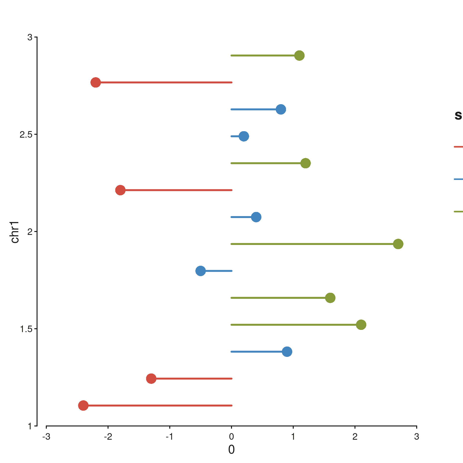

The two plots encode the same table — only the orientation of the genomic axis changes. In the flipped version the y-tick labels fall back to Mb units (the genomic yScaleFactor, matching the x-axis default) so 1.5 Mb reads as 1.5 rather than 1,500,000.

Coverage signal flipped onto the y-axis

The same principle extends to continuous signal. Below, a coverage curve is shown first in the conventional orientation, then flipped so depth runs along x and genomic position along y — useful as a narrow sidebar next to a wider browser panel.

cov_xs <- seq(1.05e6, 2.95e6, length.out = 200)
cov_gr <- GRanges("chr1", IRanges(cov_xs, width = 1),
                  depth = 0.5 + 0.3 * sin((cov_xs - 1e6) / 3e5))

seq_plot() %|%
  seq_track(data = cov_gr,
            mapping = map(x = start, y = depth),
            windows = win) %+%
  seq_area(aesthetics = aes(fill = "#4385BE",
                            color = "#205EA6",
                            alpha = 0.6, linewidth = 0.7)) -> p
p$plot()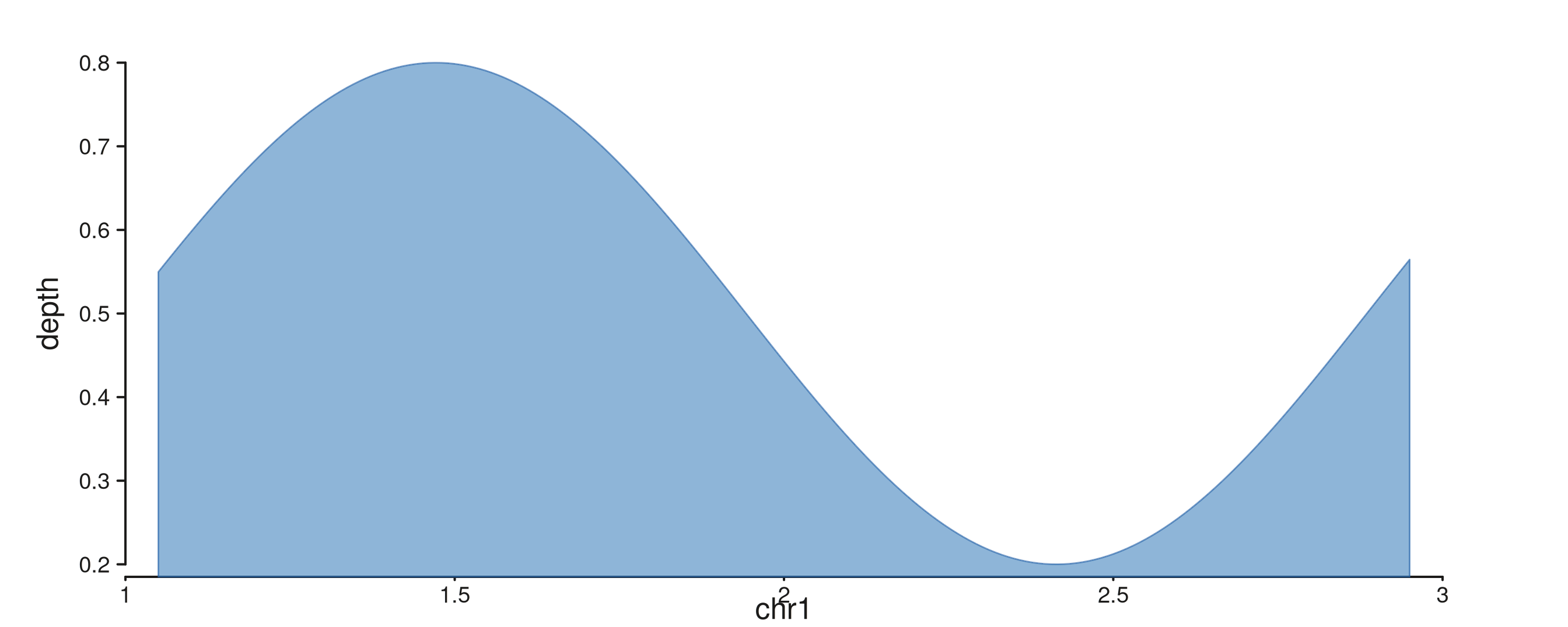

seq_plot() %|%
  seq_track(data = cov_gr,
            mapping = map(x = depth, y = start),
            windows = win) %+%
  seq_area(aesthetics = aes(fill = "#4385BE",
                            color = "#205EA6",
                            alpha = 0.6, linewidth = 0.7)) -> p
p$plot()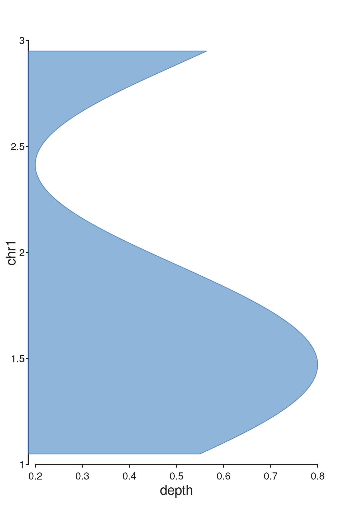

Hi-C-style rotated tiles

Rotated tiles (aes(rotate = TRUE)) place each observation as a diamond in (genomic_x, genomic_y) space — the natural representation for Hi-C contacts or any 2D genomic relationship. Both axes are genomic; pass a seq_scale_genomic() scale_y built from the distance-bin GRanges.

n_contacts <- 60
hic_win <- GRanges("chr1", IRanges(1e6, 3e6))

# Toy Hi-C: pick x-bins, then y-bins offset by a genomic distance.
x_starts <- sample(seq(1.05e6, 2.95e6, by = 2e4), n_contacts, replace = TRUE)
y_offset <- sample(seq(2e4, 8e5, by = 2e4), n_contacts, replace = TRUE)

x_gr <- GRanges("chr1", IRanges(start = x_starts,            width = 2e4),
                score = runif(n_contacts))
y_gr <- GRanges("chr1", IRanges(start = x_starts + y_offset, width = 2e4))

# Map [0,1] scores → a soft red ramp for the fill column.
score_to_color <- function(s) {
  pal <- grDevices::colorRampPalette(c("#F4A4C2", "#A02C6D"))(100)
  pal[pmin(pmax(round(s * 99) + 1, 1), 100)]
}
x_gr$fill_col <- score_to_color(x_gr$score)

seq_plot() %|%
  seq_track(data = x_gr,
            mapping = map(x = start, fill = fill_col),
            windows = hic_win,
            scale_y = seq_scale_genomic(
              GRanges("chr1", IRanges(0, max(y_offset) + 2e4)))) %+%
  seq_tile(data2 = y_gr, aesthetics = aes(rotate = TRUE)) -> p
p$plot()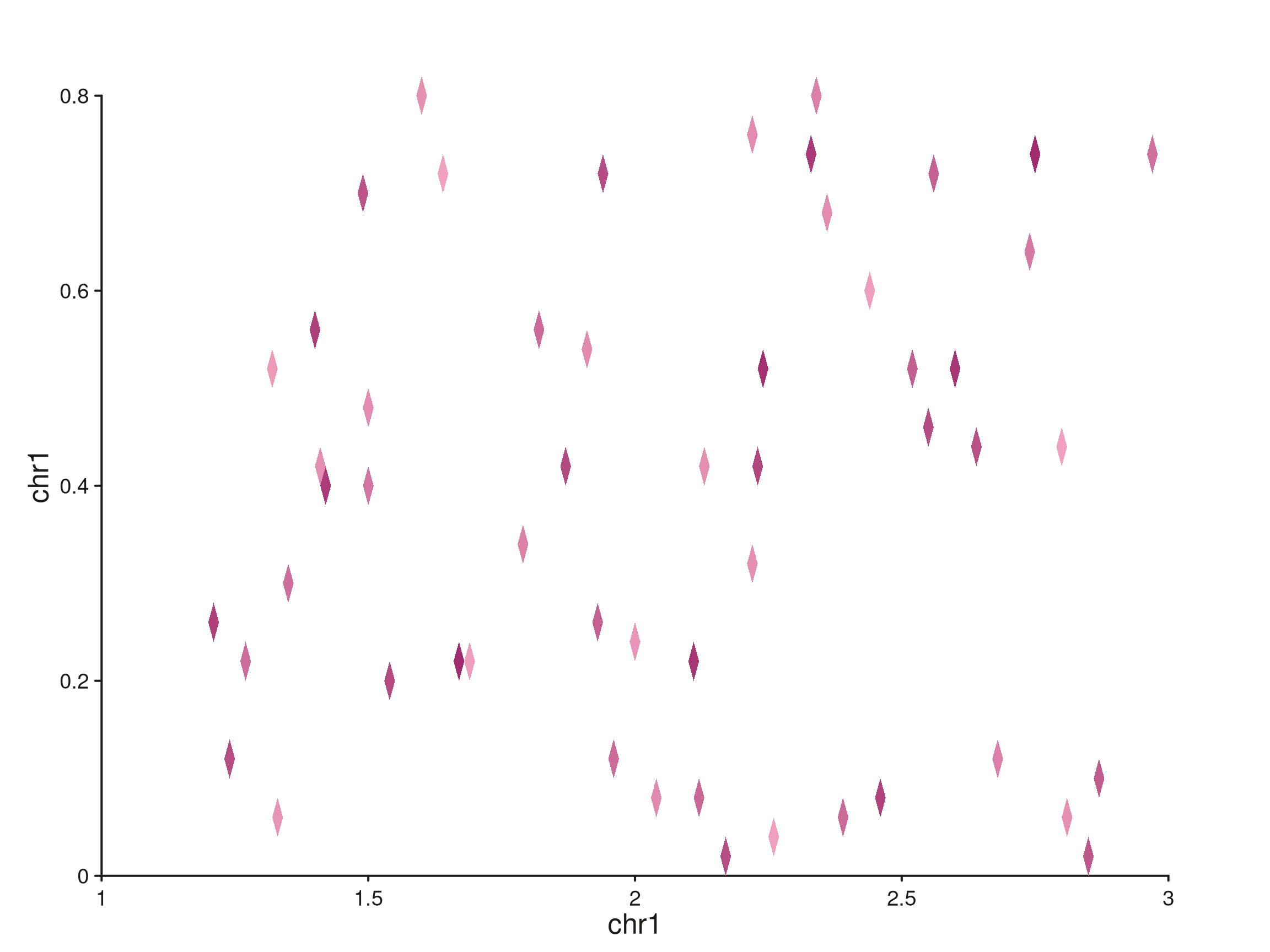

Combining multiple composites

Stack several tracks in one plot to mix composite types. Each track keeps its own data, mapping, and y-scale.

seq_plot() %|%
  seq_track(track_id = "Signal",
            data = ribbon_gr,
            mapping = map(x = start, y_min = lo, y_max = hi),
            windows = win) %+%
  seq_ribbon(aesthetics = aes(fill = "#4385BE", alpha = 0.5)) %__%
  seq_track(track_id = "Bars",
            data = bar_gr,
            mapping = map(x = start, y = score),
            windows = win) %+%
  seq_bar(aesthetics = aes(fill = "#8B7EC8")) %__%
  seq_track(track_id = "Genes",
            data = gene_gr,
            mapping = map(group  = gene_id,
                          type   = feature,
                          strand = strand_col,
                          label  = gene_name,
                          color  = color),
            windows = win) %+%
  seq_gene(map(group  = gene_id,
               type   = feature,
               strand = strand_col,
               label  = gene_name,
               color  = color)) -> p
p$plot()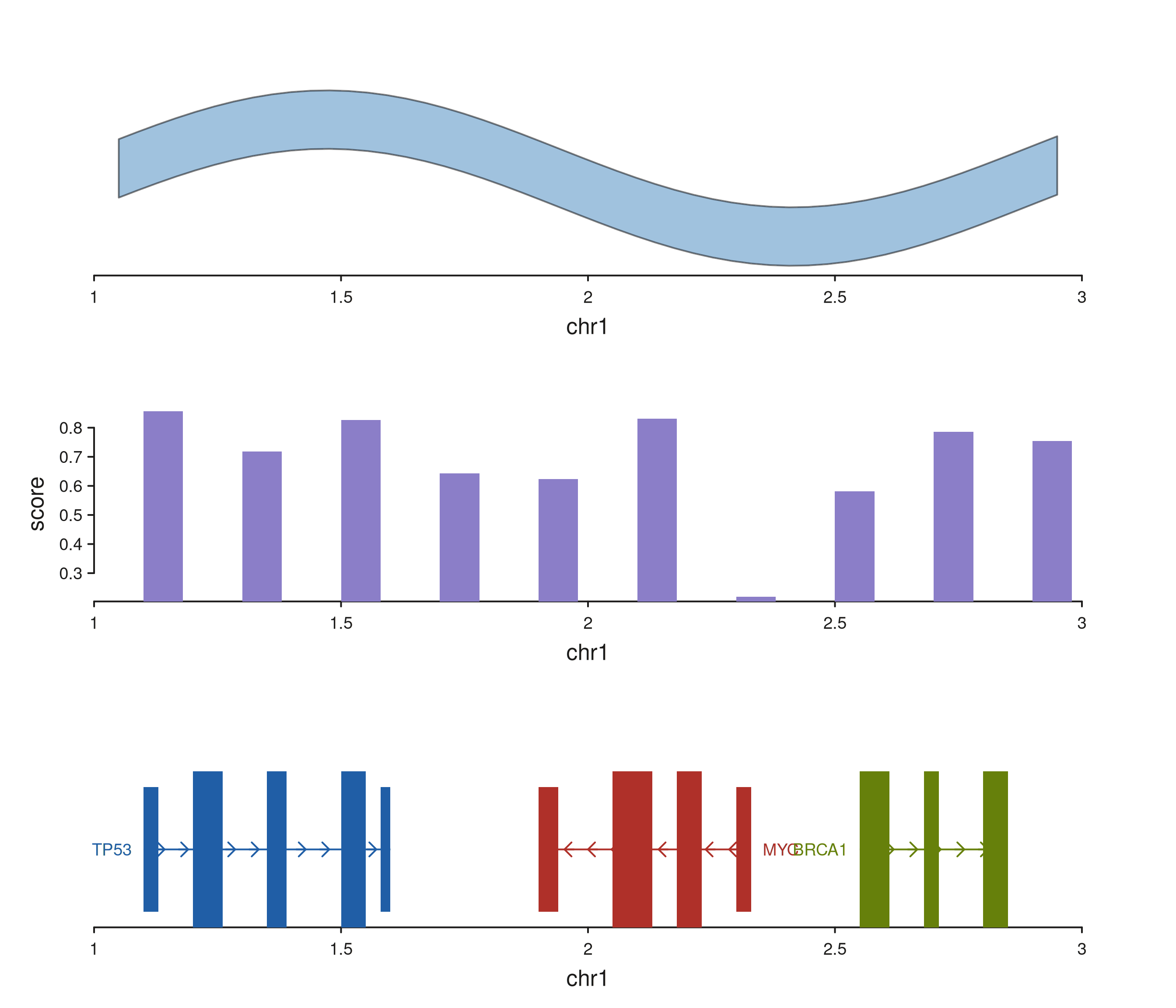

Pre-defined patchwork layouts

Passing a layout string to seq_plot(layout = ...) fixes each track’s position by track_id. Every letter in the string names a track and marks the cells it covers; # is a blank cell. seq_track(direction = ...) is ignored in this mode — position is driven entirely by the string.

The layout below reserves the top row for a signal ribbon and a density sidebar, a middle row for bars that spans the whole width, and a bottom row for gene models. seq_preview_layout() renders the layout up-front so you can verify the geometry before adding data.

layout_str <- "
AAAB
CCCC
DDDD
"
seq_preview_layout(layout = layout_str)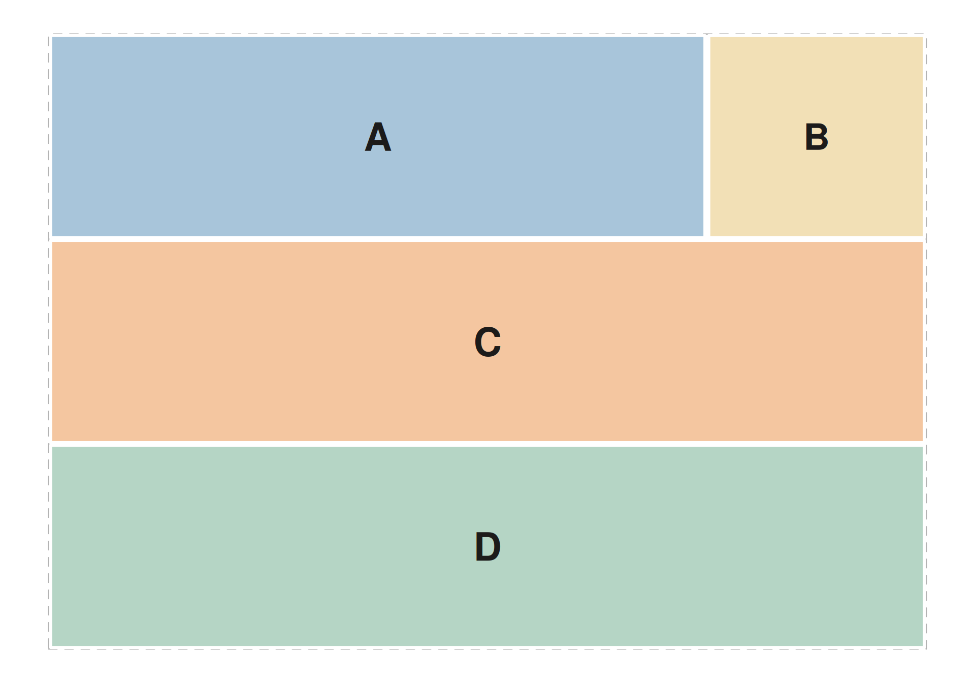

seq_plot(layout = layout_str) %+%
  seq_track(track_id = "A",
            data = ribbon_gr,
            mapping = map(x = start, y_min = lo, y_max = hi),
            windows = win) %+%
  seq_ribbon(aesthetics = aes(fill = "#4385BE", alpha = 0.5)) %+%
  seq_track(track_id = "B",
            data = dens_gr,
            mapping = map(x = start, y = score),
            windows = win) %+%
  seq_density(aesthetics = aes(fill = "#879A39", alpha = 0.7)) %+%
  seq_track(track_id = "C",
            data = bar_gr,
            mapping = map(x = start, y = score),
            windows = win) %+%
  seq_bar(aesthetics = aes(fill = "#8B7EC8")) %+%
  seq_track(track_id = "D",
            data = gene_gr,
            mapping = map(group  = gene_id,
                          type   = feature,
                          strand = strand_col,
                          label  = gene_name,
                          color  = color),
            windows = win) %+%
  seq_gene(map(group  = gene_id,
               type   = feature,
               strand = strand_col,
               label  = gene_name,
               color  = color)) -> p
p$plot()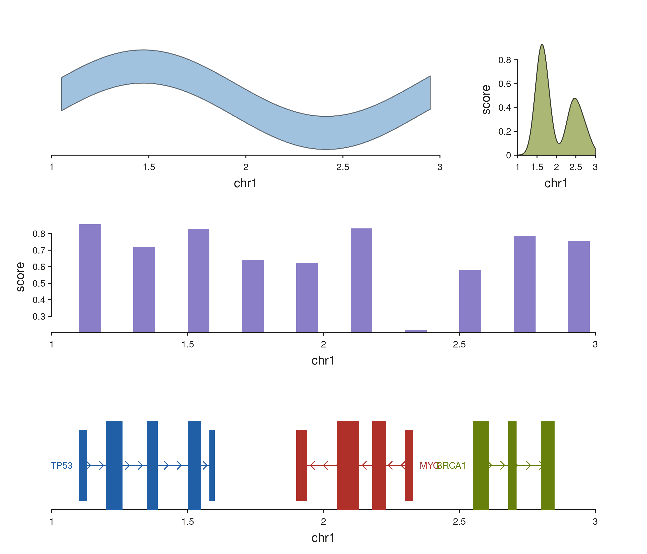

A plot that spans multiple rows

A letter’s region in the layout string is its axis-aligned bounding box, so any letter whose cells form a contiguous rectangle can span multiple rows, multiple columns, or both. In the layout below, B occupies both rows of the right-hand column while A and C share the left column and D spans the full width of the third row.

span_layout <- "
AABB
CCBB
DDDD
"
seq_preview_layout(layout = span_layout)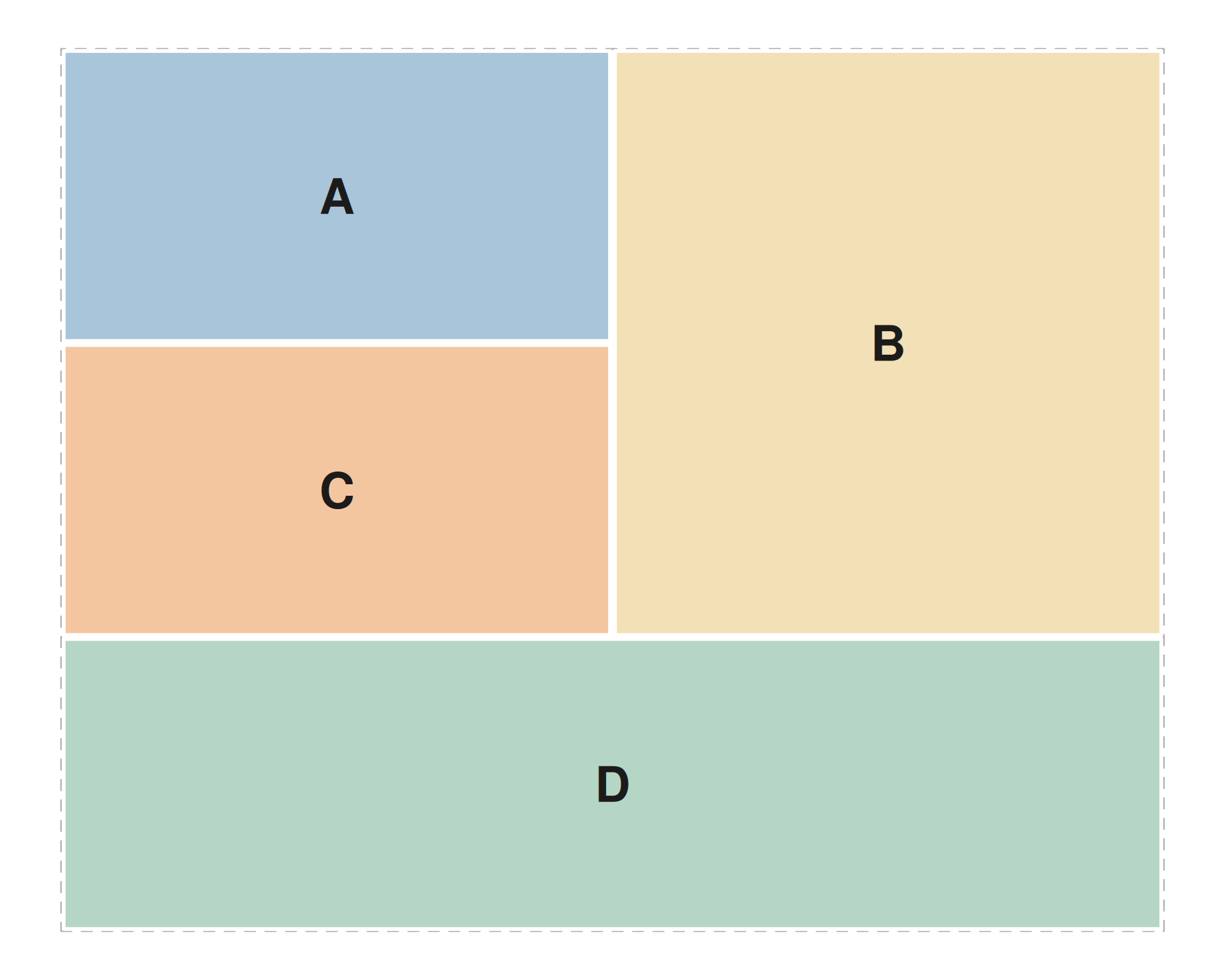

The rendered plot puts a density summary (track B) alongside two stacked detail tracks (A = ribbon, C = bars), with a genes track beneath them. Because the density track spans both rows on the right, its y-extent is the full height of A + C together.

seq_plot(layout = span_layout) %+%
  seq_track(track_id = "A",
            data = ribbon_gr,
            mapping = map(x = start, y_min = lo, y_max = hi),
            windows = win) %+%
  seq_ribbon(aesthetics = aes(fill = "#4385BE", alpha = 0.5)) %+%
  seq_track(track_id = "B",
            data = dens_gr,
            mapping = map(x = start, y = score),
            windows = win) %+%
  seq_density(aesthetics = aes(fill = "#879A39", alpha = 0.7)) %+%
  seq_track(track_id = "C",
            data = bar_gr,
            mapping = map(x = start, y = score),
            windows = win) %+%
  seq_bar(aesthetics = aes(fill = "#8B7EC8")) %+%
  seq_track(track_id = "D",
            data = gene_gr,
            mapping = map(group  = gene_id,
                          type   = feature,
                          strand = strand_col,
                          label  = gene_name,
                          color  = color),
            windows = win) %+%
  seq_gene(map(group  = gene_id,
               type   = feature,
               strand = strand_col,
               label  = gene_name,
               color  = color)) -> p
p$plot()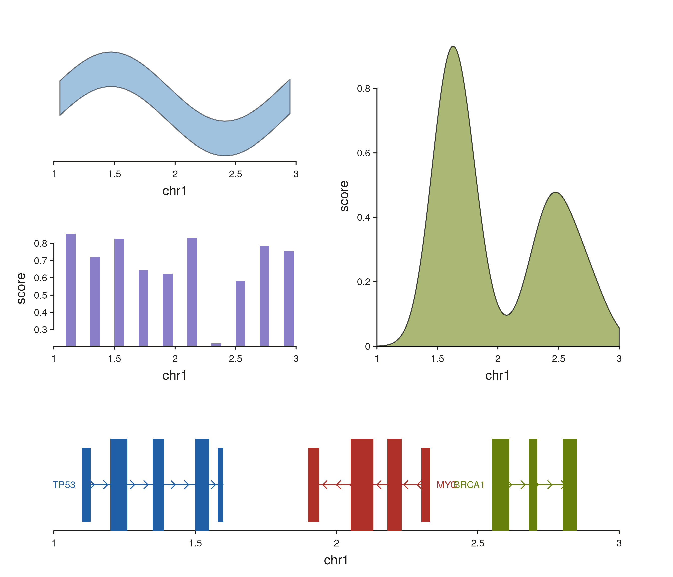

Layout-string rules:

• Every non-# letter must form a rectangular bounding box (SeqPlotR errors if an L-shape or other non-rectangle is detected).
• # cells render as empty space — no track, no axes.
• Tracks whose track_id is not present in the string are silently skipped, so the same set of seq_track() calls can be reused across different layout strings.