Getting Started with SeqPlotR

SeqPlotR builds genomic figures by composing a plot, tracks, and elements with a single %+% operator — modelled on ggplot2 but specialised for GRanges data. This vignette walks through the minimum you need to render a plot end-to-end.

library(SeqPlotR)
#> 
#> Attaching package: 'SeqPlotR'
#> The following object is masked from 'package:base':
#> 
#>     %||%
library(GenomicRanges)
#> Loading required package: stats4
#> Loading required package: BiocGenerics
#> Loading required package: generics
#> 
#> Attaching package: 'generics'
#> The following objects are masked from 'package:base':
#> 
#>     as.difftime, as.factor, as.ordered, intersect, is.element, setdiff,
#>     setequal, union
#> 
#> Attaching package: 'BiocGenerics'
#> The following objects are masked from 'package:stats':
#> 
#>     IQR, mad, sd, var, xtabs
#> The following objects are masked from 'package:base':
#> 
#>     anyDuplicated, aperm, append, as.data.frame, basename, cbind,
#>     colnames, dirname, do.call, duplicated, eval, evalq, Filter, Find,
#>     get, grep, grepl, is.unsorted, lapply, Map, mapply, match, mget,
#>     order, paste, pmax, pmax.int, pmin, pmin.int, Position, rank,
#>     rbind, Reduce, rownames, sapply, saveRDS, table, tapply, unique,
#>     unsplit, which.max, which.min
#> Loading required package: S4Vectors
#> 
#> Attaching package: 'S4Vectors'
#> The following object is masked from 'package:utils':
#> 
#>     findMatches
#> The following objects are masked from 'package:base':
#> 
#>     expand.grid, I, unname
#> Loading required package: IRanges
#> Loading required package: Seqinfo

The four primitives you need

A SeqPlotR figure is always built from these pieces:

Piece	What it does
`seq_plot()`	Creates a new plot.
`seq_track()`	Adds a genomic panel with a `windows` range.
`map(...)`	Declares data-driven aesthetics (`x`, `y`, `color`, …).
`aes(...)`	Declares constant aesthetics and theme keys.

Elements (seq_point, seq_line, seq_area, …) are drawn inside a track. The %+% operator chains everything together and dispatches on the right-hand side’s class.

A first plot

win <- GRanges("chr1", IRanges(1, 1e6))
gr  <- GRanges("chr1",
               IRanges(start = seq(1e4, 9.9e5, length.out = 200), width = 1),
               score = sin(seq(0, 6*pi, length.out = 200)) +
                       rnorm(200, 0, 0.1))

p <- seq_plot() %+%
  seq_track(data = gr, mapping = map(x = start, y = score), windows = win) %+%
  seq_point(aesthetics = aes(color = "#205EA6", size = 0.4))

p$plot()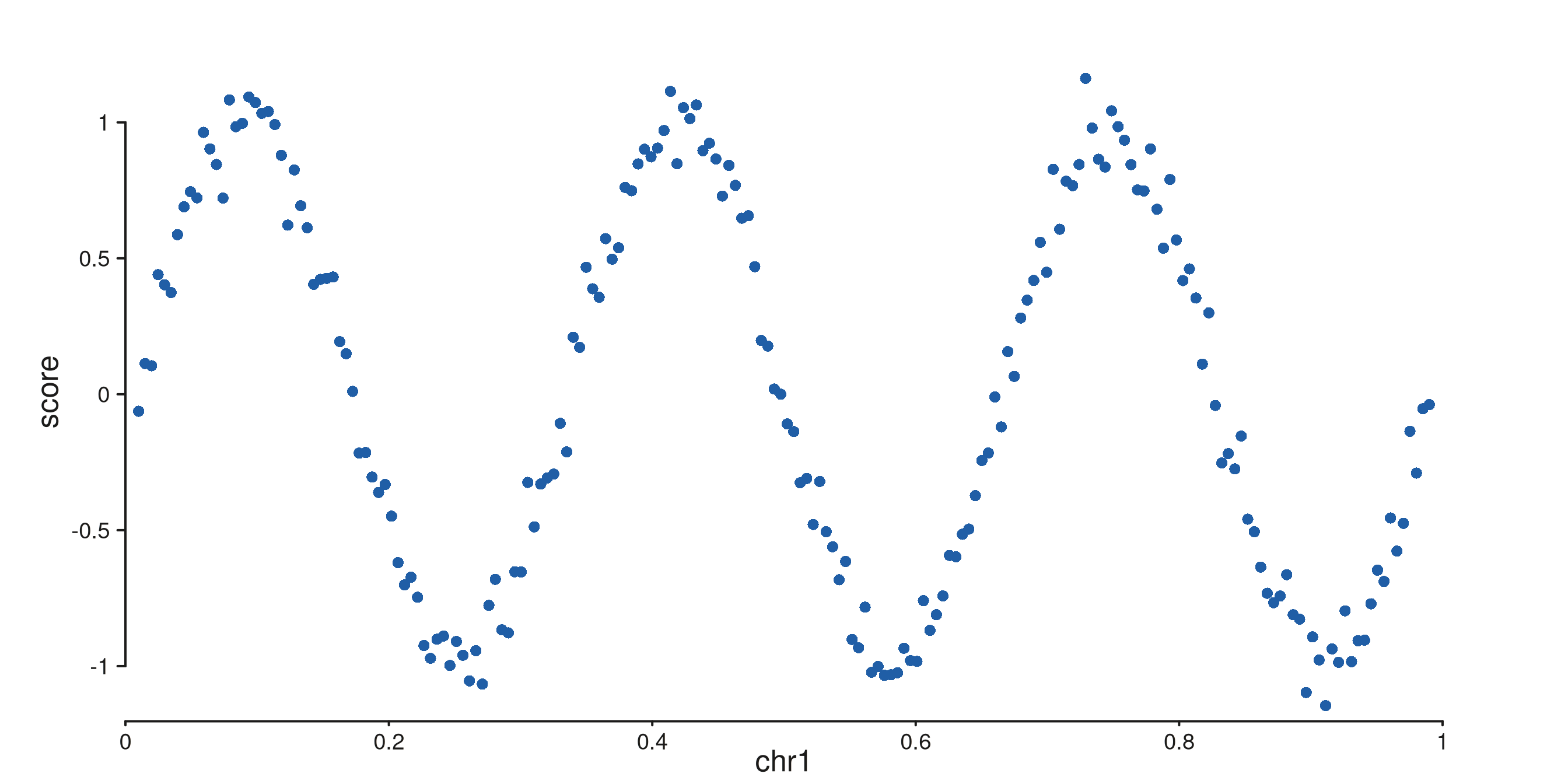

The track holds the defaults (data, mapping, windows); the element seq_point() inherits them.

Layering several elements in one track

%+% on a plot adds elements to the most recently added track, so two elements in a row draw on top of each other:

gr_line <- GRanges("chr1",
                   IRanges(seq(1e4, 9.9e5, length.out = 200), width = 1),
                   value = cumsum(rnorm(200)) * 0.05)

p <- seq_plot() %+%
  seq_track(data = gr_line, mapping = map(x = start, y = value), windows = win) %+%
  seq_area(aesthetics = aes(fill = "#92BFDB", color = "#205EA6", baseline = 0)) %+%
  seq_point(aesthetics = aes(color = "#205EA6", size = 0.3))

p$plot()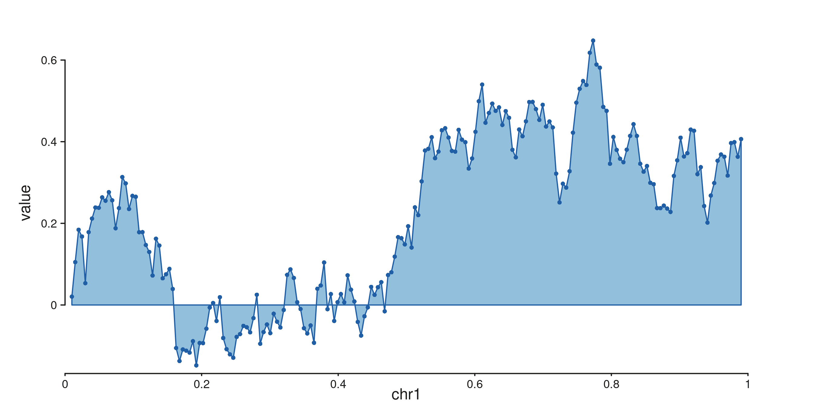

Two tracks side by side: `%|%` and `%__%`

%|% and %__% are convenience aliases for %+% that set direction = "right" or direction = "under" on the track they introduce:

gr_a <- GRanges("chr1", IRanges(seq(1e4, 9.9e5, length.out = 100), width = 1),
                score = rnorm(100))
gr_b <- GRanges("chr1", IRanges(seq(1e4, 9.9e5, length.out = 100), width = 1),
                score = rexp(100, rate = 0.5))

p <- seq_plot() %|%
  seq_track(data = gr_a, mapping = map(x = start, y = score),
            windows = win, track_id = "A") %+% seq_line(aesthetics = aes(color = "#205EA6")) %__%
  seq_track(data = gr_b, mapping = map(x = start, y = score),
            windows = win, track_id = "B") %+% seq_area(aesthetics = aes(fill = "#F9AE77"))

p$plot()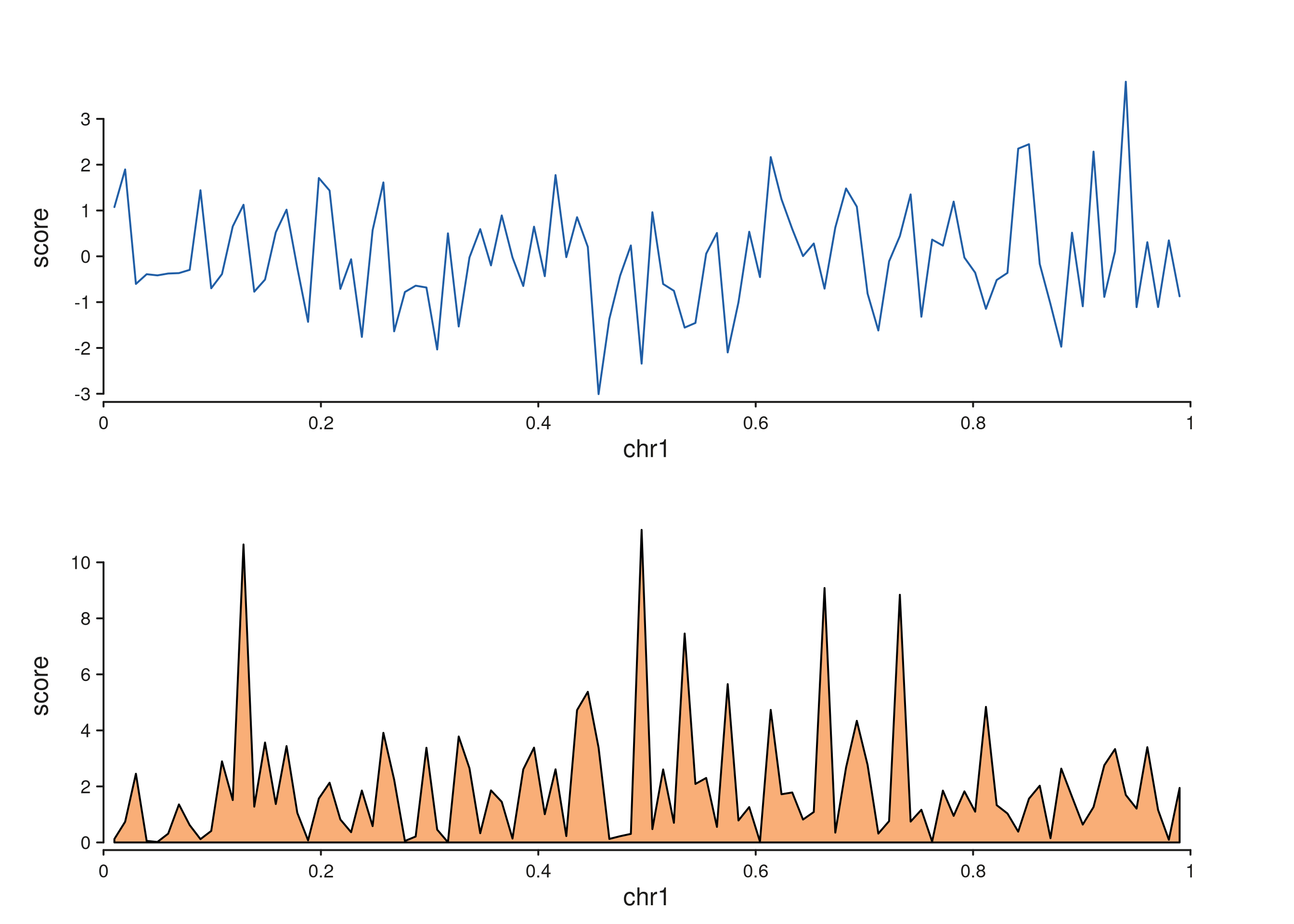

Printing

seq_plot carries an S3 print method, so a bare expression in a script or knitr chunk auto-renders — p$plot() is equivalent.

Where to go next